Introduction

Many finance academics have long touted the superiority of the real options valuation approach for capital investment analysis over the traditional discounted cash flow method. The classic academic text on real options is Dixit & Pindyck (1994). They dedicated their book to “The Future” as they foretell of a time when real options analysis is the dominant paradigm for investment valuation and capital budgeting. With the rise of data science, and businesses becoming more comfortable with quantitative approaches to decision making, I suspect that real options analysis will become a standard technique in the financial analyst’s arsenal. Additionally advances in both algorithms and computing power allow the use of simulation to solve real options problems without the use of any sophisticated mathematics.

So I thought I would post a basic real options model that is solved using an approximate dynamic programming technique called Least Squares Monte Carlo simulation (LSM). This algorithm was introduced in an influential paper for the valuation of American style options, Longstaff & Schartz (2001). However the algorithm is very general and highly adaptable to many real options situations. Within the real options framework it has been applied to valuing pharmaceutical R&D, gas storage facilities, and renewable energy just to name a few. For a more extensive list see Nadarajah, Margot, & Secomandi (2017).  In future posts I plan on reconstructing several more examples including presenting a real estate case study. This is an exciting area of finance as it has the potential to greatly improve business decision making.

The example in this post is a natural resource investment, specifically the mine valuation model from a classic real options paper, Brennan & Schwartz (1985) (henceforth “B&S”). Since there are several ways to extend the LSM algorithm to multi-state switching options, the LSM variant that I use is from Cortazar et al (2008) (CGU) which also solves the B&S mine valuation model. For an alternative approach to extending LSM to real options models, see section VIII of Sick & Gamba (2010), which includes a nice and simple example.

Before I discuss the model’s details, let’s do a brief review of real options and discuss several methods used for solving them.

Real Options Review

Real options are models of managerial flexibility, which can be defined as the value created by the future decisions that managers possess in response to both economic and non-economic uncertainties. Real options grew out of academic research in valuing financial options. Researchers noticed that the future decisions of a company could be conceptualized as call and put options much like the options that trade on financial exchanges.

For instance in the mine example below, at each decision date the operator has an option to abandon the project (if abandonment hasn’t already occurred), as well as options to change the operating mode of the project from open to close or closed to open depending upon the current state. This insight allows managers to use option pricing techniques and dynamic programming in valuing real assets and business decisions.  Most real options situations can be modeled as American or Bermudan options because they possess early exercise features. (The difference between American and Bermudan options is that early exercise can occur at any time prior to expiration with an American option but only on a discrete number of dates for the the Bermudan option. In practice, numerically, we will solve a Bermudan option as an approximation to an American option.)

In contrast to real options analysis, the tradition and dominant method of capital budgeting and capital investment valuation is discounted cash flow analysis (DCF). The most popular variants of DCF being the IRR and the NPV. However the primary drawback of DCF is that it is a static method that assumes that all decisions are made at a single point in time and that managers can make no future operational changes.  To be concrete let’s compare the real options value, ROV, and the NPV formulas. The NPV decision rule, which is to invest if the NPV is positive, has the following form:

where is the discount factor in period and is the period expected net cash flows.

In contrast, the real options value can be represented by the following cash flow stream:

where the ROV equation includes a maximum operator over which a sequence of actions, , must be chosen. is the net cash flow in time period , but now the net cash flows are functions of the actions taken in each time period.  Thus the critical difference between the NPV and the ROV is the ability of the real options method to account explicitly and quantitatively for managerial decision making. This ability to alter decisions in future time periods increases the value of an investment in many situations.

Solving Real Option Models

In practice real options models are solved using a variety of different approaches with the most popular being: binomial trees, finite difference methods (FDMs), and Monte Carlo simulation. Binomial trees and FDMs have the advantage of being computationally efficient and accurate when there is a single source of uncertainty. However neither method scales well to handle multiple sources of uncertainty.  They also include implicit assumptions on the modeled probability distribution, e.g. a binomial tree approximates a lognormal distribution. These limitations have led to an interest in using simulation based methods for option valuation. Simulation can, at least in theory, be used to value any number of uncertainties with few restrictions on the underlying distribution.

How does simulation work to solve the ROV cash flow equation above? Finding an entire sequence of actions that maximizes the ROV equation at once can be mathematically difficult. So we first need a tractable mathematical formulation of the problem that we can solve numerically. Fortunately researchers, such as Bellman (1957), noticed that problems like the ROV equation can be decomposed into a problem with two components: the immediate value of an action and a function representing the value from all future decisions given the immediate action. This technique is called dynamic programming and has applications throughout applied mathematics, operations research, and finance. With a dynamic programming formulation the ROV equation becomes:

where is the value of the project in period , is the period net cash flow as a function of the action taken in that period, and is the discounted expected future value of the project given the decision today.  (Note that my formulation above is simpler than what occurs in practice and in the literature where there are state variables that are functions of the action. However I want to focus on the primacy of actions and decisions. See Powell (2011) chapter 3 for a general overview of dynamic programming and relevant mathematical proofs.)

Now with this new formulation of the ROV equation, we can employ a solution strategy called backward induction to solve the problem. Backward induction means that we start in the last time period (when the term is zero since there is no future value) and solve for the best final action, and then work backgrounds through time to the initial value. This approach is the basis of the LSM algorithm.

The difference between using a generic backward induction algorithm and LSM relates to the nature of using simulation to model the uncertain variables. A long cited obstacle with using Monte Carlo simulation for options with early exercise features, like the mine example here and most real options, is that MC simulation moves forward in time. However dynamic programming moves backward in time.  This means that when using simulation with backward induction, backward induction uses simulated information about the future in determining the optimal decision. Unfortunately this is a form of perfect foresight bias that, if not corrected, leads to errors in valuing real options.

The LSM algorithm was developed to handle this bias. In short the LSM can be thought of as a form of bias reduction by using regression analysis. To put it more formally, LSM minimizes the valuation bias by using Ordinary Least Squares estimation of the cross section of simulated values in the current state to estimate the conditional expectation of the discounted future value function, the term above. Thus we are reducing the impact of foresight bias by using the value today of the uncertain variables to predict tomorrow’s value function via linear regression. Using the LSM approach with a sufficient number of Monte Carlo runs and an appropriate set of basis functions for the regression, the estimated value should converge to the true value. (For a technical discussion of the LSM algorithm’s mathematical properties, like convergence, see Clément et al. (2002).)

The Mine Example

As mentioned above the example here uses the core assumptions of Brennan & Schwartz (1985) to value a mineral concession while accounting for the mine owners ability to open a closed mine, temporarily close an open mine, and the option to abandon the mine completely.

As with my other posts so far, I have used the excellent Analytica modeling language to build this model. You can download the mine example here, and the free version of Analytica here. For open source alternatives see the popular data science languages Julia, R, or Python. Personally, of the three, Julia is becoming my favorite due to its outstanding speed and its clean syntax. I will probably do some Julia examples in the future. (In the context of dynamic programming problems, see this paper for a comparison between several languages; Julia comes out on top compared to R and Python by a substantial margin.)

Now let’s turn to the mining model. I always like to start with the input panel containing the model assumptions. The ability to easily create these panels is a great feature of Analytica. Help balloons are enabled, so just hover your cursor over an input field and a description of that variable will appear.

The inputs under the Project header are the basic assumptions regarding the copper resource including the switching costs of opening and closing a mine, the annual maintenance cost of a closed mine, and the unit cost of production.  In this model the annual output, and thus the output per period, are constant for the given number of decision epochs per year. However having output be a decision variable is certainly something that can be accommodated within the dynamic programming framework.

The Resource assumptions are the inputs for the only source of uncertainty in this model, the copper price over time.  The model simulates the risk neutral (risk-adjusted) copper prices using geometric Brownian motion. This simulation accounts for the cost inflation of production and switching costs, the convenience yield of the copper, and the copper price’s volatility. Of course GBM is used here only for example purposes. More realistic copper price dynamics are explored in Cortazar et al (2008). Additionally Abel Sabour & Poulin (2006) extend the B&S model to include seven different minerals, each with their own stochastic price process.  Several of the metals in their paper have mean reversion processes, which may be more realistic in many settings. As mentioned above, when there are multiple sources of uncertainty, simulation is the way to go.

The tax assumptions account for the property tax of the property and the income taxes.

The final section of inputs are the assumptions for the simulation and the basis functions for the the regression analysis. The sample size is the number of simulated price paths for each run of the model. Increasing the sample size is important to achieve convergence to the true value. The polynomial order assumption is used to determine the polynomial that will approximate the discounted expected value function in the regression analysis. The decision epochs variable determines the number of times per year that a switch in state can be made. In the parlance of American options, the decision epochs are the number of exercise points each year.

Lastly, a choice menu allows the basis functions used in the OLS regression to be either ordinary power series or Laguerre polynomials. While power series are common in the literature, Laguerre polynomials are more theoretically satisfying. Their drawback is that they may be numerically unstable is some cases, see Boogert & de Jong (2008), and tend to take longer to compute. Choosing basis functions is a bit of an art that really depends on the underlying uncertainty being simulated. A more complete economic model, like using futures prices to approximate the value functions is a good alternative to polynomial approximation as demonstrated in Cortazar et al. (2008), section 4.3. For an excellent textbook treatment of approximating functions see Judd (1998) chapter 6.

Lastly, a note on the implementation in Analytica: to conserve memory the Iterate function was used for the backward induction process instead of the more satisfying Dynamic function. However to determine the optimal switching and abandonment operating policies, Dynamic can be used to store the decision paths.

The Results

So for demonstration purposes I set the model to perform 5 runs (starting from different random seeds), each with 30,000 sample paths, and then averaged them together. The model used Laguerre polynomials of order 4 to approximate the discounted expected value function. Three decision epochs were used for each year. The results are the following:

For comparison below are the results from B&S (center column) and Cortazar et al. (2008):

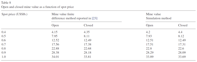
B&S used a finite difference method, while Cortazar et al‘s algorithm is the algorithm I used in the example model. Overall I think the example model’s results are good. In experiments averaging more runs of the model, the values continued to converge to B&S’s results. I attribute the difference in values between the model and B&S/Cortazar primarily because of the small number of simulations in each run of the model. Cortazar et al used 50,000 paths for their simulation. Since Analytica 101 limits indexes to be 32,000 elements in length, as mentioned above, I only used 30,000 per model run. This limited the information used in the regression.

For another comparison, below is a graph of the open state in the initial period compared with Brennan & Schwartz emphasizing the small difference in results:

Conclusions

Overall the model seemed to work well to approximate the mine valuation model of Brennan & Schwartz. The biggest hurdle with the model was the slow computation rate of the Monte Carlo simulation. Additionally for a model to be used in practice a more realistic price process would have to be used. Uncertainty assumptions over other variables such as operating costs can also be added.

Real options models have a lot to lend business decision makers and I hope that they become more utilized in practice. Time will tell. As always if you have any question feel free to email me.

References

1. Bellman, R. (1957) Dynamic Programming, Princeton University Press (Amazon)
2. Boogert, A. & Cyriel de Jong. (2008). Gas storage valuation using a Monte Carlo method. Journal of Derivatives, 15(3), p. 81-98 (PDF)
3. Brennan, M., & Schwartz, E. (1985). Evaluating Natural Resource Investments. The Journal of Business, 58(2), 135-157 (PDF)
4. Clément, E., Lamberton, D. & Protter, P. (2002). An analysis of a least squares regression method for American option pricing. Finance Stochast 6, 449–471. (PDF)
5. Cortazar, G., M. Gravet, & J. Urzua. (2008). The valuation of multidi-mensional American real option using the LSM simulation method. Comput. Oper. Res., vol. 35, pp. 113–129. (PDF)
6. Dixit, A. & Pindyck, R. (1994) Investment Under Uncertainty, Princeton Press. (Amazon)
7. Judd, K. (1998). Numerical Methods in Economics, MIT Press. (Amazon)
8. Longstaff, F., & Schwartz, E. (2001). Valuing American Options by Simulation: A Simple Least-Squares Approach. The Review of Financial Studies, Pages 113–147. (PDF)
9. Powell, W. (2011). Approximate Dynamic Programming, Princeton Press. (Amazon)
10. Nadarajah, S., Margot, F., & Secomandi, N. (2017). Comparison of Least Squares Monte Carlo Methods with applications to energy real options. European Journal of Operations Research, 256, pp. 196-204. (PDF)
11. Sabry A. Abdel Sabour & Richard Poulin (2006). Valuing Real Capital Investments Using The Least-Squares Monte Carlo Method. The Engineering Economist, 51:2, 141-160, DOI: 10.1080/00137910600705210
12. Sick, G. & Gamba, A. (2010). Some Important Issues Involving Real Options: An Overview. Multinational Finance Journal. Vol. 14, No. 1/2, p. 73-123. (PDF)