Recently I have been developing a credit risk model, so I thought I would post a scaled down version for anyone interested in using Monte Carlo simulation to analyze credit risk. As the global coronavirus pandemic has made clear, financial models need to explicitly account for uncertainty and rare events and Monte Carlo simulation is the perfect tool for the job.

The credit risk model presented here is standard. It combines a migration analysis using credit rating migration matrices with a default and recovery analysis. A Gaussian copula is incorporated into the model to handle dependencies between the assets. Like most models of this kind it descends from the classic CreditMetrics approach that JP Morgan published in 1997. Here is the most recent CreditMetrics technical document that I could find. The discussion is quite lucid and instructive. Hull (2018), p. 486, provides a concise introduction to the CreditMetrics method.

Like CreditMetrics, the model here estimates expected and unexpected losses and two measures of tail risk, the popular Value-at-Risk and Expected Shortfall Risk. In addition to the CreditMetrics document, the other primary reference for the model is Ramaswamy (2004). This excellent book is a comprehensive approach to corporate bond portfolio management for practitioners and covers many issues not addressed here. Additionally, the book suggests several adjustments to the CreditMetrics method that I include in the model here.

Any interested reader can download the model at this link. It was constructed in Analytica so you will need the free version (here) to view and alter the model’s inputs. Analytica continues to be my favorite financial modeling environment, but credit risk models are implemented in all the major data science languages of R/Python/Julia. If you haven’t tried Julia, then I highly recommend it. It is a much faster and sleeker alternative to Python and R. When not using Analytica, Julia is my preferred choice.

Credit Risk Background

Fixed income investments face several types of risks. Blackrock identifies four primary categories of fixed income risk: interest rate risk, inflation risk, liquidity risk and credit risk. Additionally, I would also include economic and event risk, which affects entire sectors of the economy. While each of these risks is important, the focus here is on credit risk. Extending the model to account for these other risks is fodder for another time.

So what is credit risk? The Basel committee on Banking Supervision defines credit risk as “the potential that a bank borrower or counterparty will fail to meet its obligations in accordance with agreed terms.” This is a very general definition and it is meant to be. Credit risk is broader than the banking context and is present in just about any economic transaction when payment is not contemporaneous with the provision of the good or service being exchanged. As an example, the receivables for a plumbing company are subject to credit risk. For our purposes, credit risk is modeled as the change in the credit quality of a corporate bond issuer. Quality refers both to default risk and to a change in the market’s perception of a possible default as captured by the obligor’s credit rating.

Complications also arise once the situation changes from a single asset with credit risk to a portfolio of such assets. Within a portfolio the credit risks between assets will invariably be interdependent. This dependency between the assets needs to be explicitly taken into account otherwise the simulation and analysis will not produce informative results and statistics.

Furthermore traditional statistics like the mean and standard deviation may be misleading if they are the only statistics used in analyzing a credit portfolio. This is because credit loss distributions are asymmetrically skewed on the losses side of the ledger so that these statistics do not provide adequate information concerning tail risks. The best that a bond can do is meet its obligations. But a bond that moves into default or whose issuer experiences a negative change in their credit rating can have a dramatic impact on a portfolio’s value. For example here is the simulated loss distribution for the example portfolio discussed below (gains are negative and actual losses are positive, although the term “losses” refers to both):

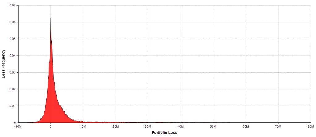
Note the skewed distribution to the right indicating the potential for large losses. In this example the minimum loss (gain) is about $-8.232M and the maximum loss is $71.74M, a massive hit to the portfolio’s value.

For the rest of the blog post I will walk through an example credit analysis for a portfolio of corporate bonds. The data is taken from Ramaswamy (2004), chapter 6. Using this data allows readers to see some external validation for the model. However, almost all the the inputs can be altered directly via the input panels which the user will see upon opening the model.

Note also that while this model is focused on corporate bonds the general principles of this approach apply to most fixed income securities. Chapter 4 of the CreditMetrics technical document linked above has a nice discussion of how to handle a variety of different fixed income securities including traditional corporate bonds, bank facilities (e.g. letters of credit) and market based instruments such as swaps.

The Model

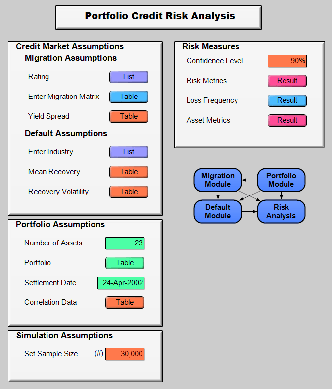
Below is the assumptions and results panels for the model. Analytica offers easy to use input and output panels which act as interfaces between users of the model and the model’s details. A help balloon with a description of the input variable will appear if the user hovers their cursor over the variable name.

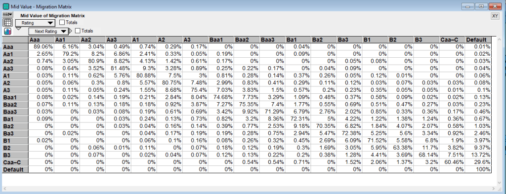
I won’t walk through all the assumptions above, most of which are simply input tables like the Enter Migration Matrix table below. This matrix represents the probability of a rating moving from the row rating to the column rating. So the probability that an asset rated Aa1 moves to rating Aaa is 2.65%.

Once the other assumptions are entered, then the portfolio details can be completed in the Portfolio table. As mentioned above the data comes from Ramaswamy (2004). The sample portfolio is 23 corporate bonds each from a different obligor. (The reason that these are different obligors is that this model does not consider the case of cross default clauses, which declare all debt issues of an obligor in default if one issue defaults.)

The data for each bond in the portfolio is entered into the Portfolio table:

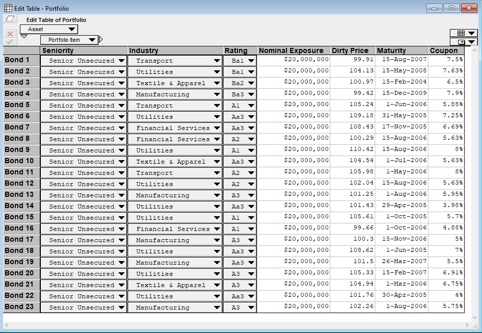
The seniority and industry inputs select the mean and standard deviation used during the recovery rate simulation. The rating is the credit rating of the obligor based on the rating system used. A user can enter their on rating system on the general inputs panel above. The nominal exposure is the total face value exposure. The Dirty Price is the quoted price plus accrued interest as a percent of face value. The maturity date and the coupon rates are the last items entered.

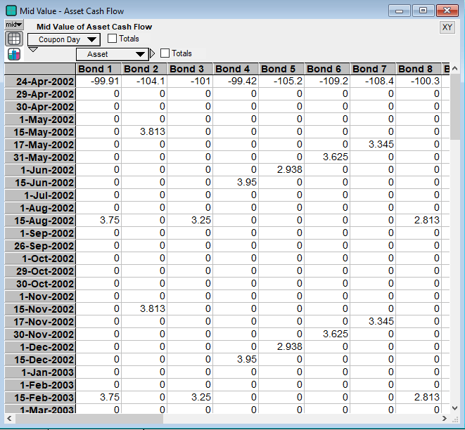
Once all of these inputs have been entered, then the model will first calculate each of the coupon payments at the appropriate dates between the settlement date (the day when the analysis is performed) and the maturity date for each bond. Below are the cash flows for the first several bonds and coupon dates starting at the settlement date. Note that the coupons are paid at six month frequencies as is standard for a corporate bonds.

From these cash flows the model will then calculate the yield to maturity, the modified duration and the convexity, which are below:

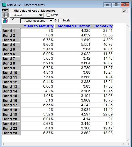
The modified duration and convexity are measures of interest rate sensitivity for an asset. They estimate how much an asset’s price changes for a change in yield. When an asset migrates to a different credit rating its yield will change to reflect the new credit risk. The classic CreditMetrics model involved calculating forward yield curves for each credit rating and then discounting back the coupons of each asset by their credit risk adjusted discount rates. However since yield curve construction can be difficult and a source of model noise, Ramaswamy (2004) suggests using the modified duration and the convexity to provide a second order approximation of the price change when the rating changes. With this approach there is no need to construct yield curves. The yield spreads used for each credit rating are the spreads on the settlement day, which are known (and entered into the model above in the Yield Spread input). This approximation of the price change using the modified duration and convexity is the approach that this model takes. However to see an example of a yield curve construction, see Saunders & Allen (2010), chapter 9, page 195. Also see Luenberger (1998) chapter 3 for a discussion and derivation of duration and convexity more generally.

Now that how the model handles price changes has been described I will turn to how the model incorporates rating migrations and default. Since Analytica is a visual modeling language I will post the influence diagram and discuss how things are calculated. To see the actual formulas just look at the definitions of each node on the diagram.

Migration Analysis

Credit migration is the change in credit rating that can occur for each asset in the portfolio over the risk horizon. The risk horizon is assumed to be one year here. To recap, any change in rating results in a change in yield since different yields have different spreads above the risk free rate based on their perceived credit risk. This change in yield changes the price of the asset resulting in a loss for the portfolio, where negative losses are gains in portfolio value and positive losses are actual losses of value.

In this model, migration analysis is built around two key inputs, the correlation data and the migration matrix. See the influence diagram below. The orange trapezoid nodes represent assumptions and are entered into the model by the user on the inputs and assumptions panels.

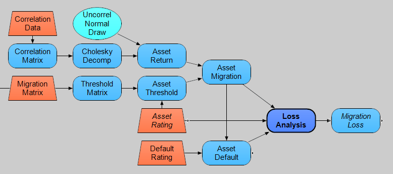
The correlation data is the asset return correlation coefficient for each asset pair in the portfolio. I won’t get into how to estimate asset correlations as that is more art than science and there are many different approaches. The model here assumes that some sort of factor analysis has been used to derive the correlations between the asset returns. These asset returns serve as a proxy for correlated credit events because correlated credit events are difficult to estimate directly. See the CreditMetrics document, chapter 8, and Ramaswamy (2004), chapter 6, for extensive discussions on how to derive estimates of loss correlations.

The Asset Return variable is then the simulated correlated asset returns. These are standardized asset returns having a zero mean and standard deviation of one. The model here only needs the correlation data and does not depend on other individual asset return statistics. Asset Return is generated using a Gaussian copula method that decomposes the correlation matrix and then combines it with uncorrelated draws from a multivariate standard Normal distribution that represents the uncorrelated standardized asset returns for each asset.

The normality assumption is not restrictive in the sense that many other distributions can be used. See Trueck & Rachev (2009), chapter 10, for a discussion of copulas, their usage with migration matrices and other possible distributions. Hull (2018) is also very instructive on copulas and the CreditMetrics approach. Ramaswamy (2004), chapter 8, applies the Student’s t distribution to the example portfolio data used in this post.

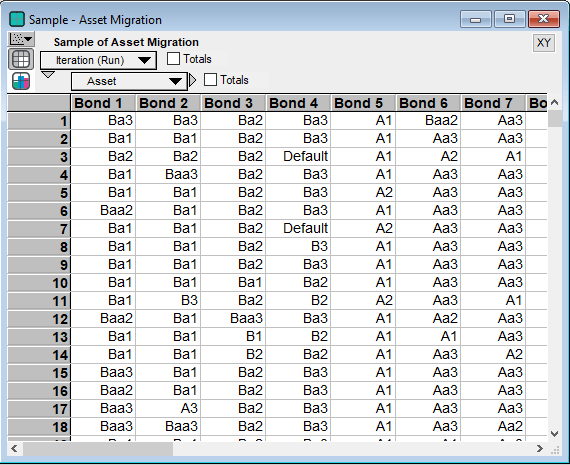
Several simulation runs for the correlated asset returns are below.

The other piece of the migration analysis starts with the Migration Matrix, which is the matrix of transition probabilities between ratings. The migration matrix for this model is shown (again) below. Just to reiterate, the probability in each cell is the probability of moving from the row’s rating to the column’s rating over the risk horizon.

As can be seen from the migration influence diagram above, the migration matrix is used to create the Threshold Matrix variable, which contains the threshold standardized asset return values that determine the credit rating of each asset at the risk horizon. This variable uses the inverse normal distribution to map the transition probabilities to the threshold values. The Asset Threshold (below) is simply the threshold values for each asset given their initial ratings.

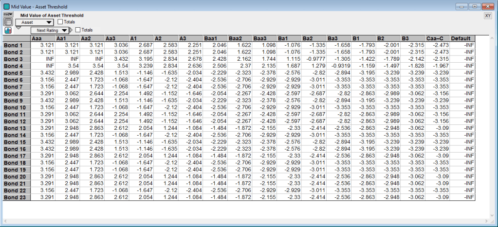
The threshold values represent the asset returns that are the minimum return needed to transition into the column’s credit rating. So for example, if Bond 1’s asset return is greater than or equal to 2.583 but less than 2.687, then its credit rating will migrate from the initial Ba1 rating to the A2 rating.

Combining the Asset Threshold variable and the Asset Return variable gives us the migrations for each simulation run of the portfolio. Below are several of the bonds and their migrations on different simulation runs. For instance during simulation run 6, Bond 1 has an Asset Return value of 2.02 (see above). Then from the Asset Threshold table we see that 2.02 is greater the Baa2 threshold of 1.622 but less than the Baa1 threshold of 2.046. Hence Bond 1 moves from the initial rating of Ba1 to Baa2 on run 6.

Once the migrations are determined, then for non-defaulting assets, the appropriate price change is calculated using the current yield spreads, the modified duration and convexity as discussed above.

This is just the briefest of overviews for how credit migration is simulated. The CreditMetrics and Ramaswamy (2004) discuss this process in more detail. See also Trueck & Rachev (2009) for a very nice discussion of copula methods and their use in ratings migration analysis.

The last piece of the credit risk puzzle is what happens on default. I discuss this next.

Default Analysis

Default occurs when an asset migrates to the default state of the rating system used. Different ratings systems have slightly different definitions of default and what constitutes a default. However the core concept of default is that the obligor has economically impaired the bondholder through the obligor’s inability to meet the asset’s payment schedule.

The default and recovery model here is the standard CreditMetrics approach. A Beta distribution is simulated to determine the recovery rate, which is one minus the loss given default. Recovery rates are the percentage of face value that the bondholder will receive if default occurs.

The parameters for the Beta distribution are derived from historical recovery rate statistics, specifically their means and standard deviations segmented by industry and seniority. Thus different industries and seniority levels can have different recovery means and standard deviations. These are altered on the assumptions panel (above). For this model the recovery mean is 47% and the standard deviation is 25% across all industries and seniority levels. These statistics are for example purposes only. See Altman & Kishore (1996) for a good starting point to explore the literature on historical recovery rate statistics. The influence diagram for the default analysis is below.

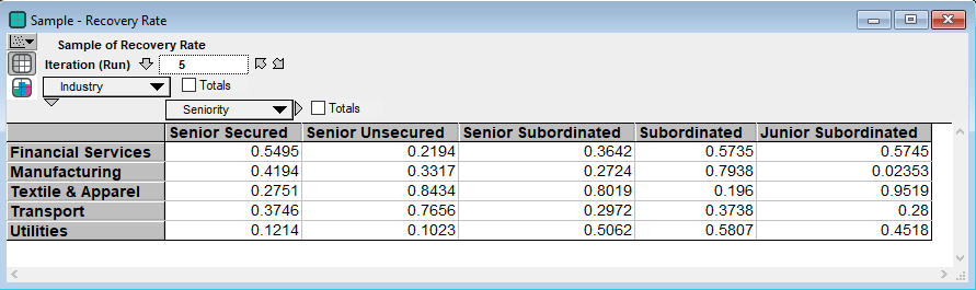
The Recovery Rate node is the simulated recovery rates for each seniority level and industry on each run of the simulation. Below are the simulated recovery rates for run 5 of the simulation:

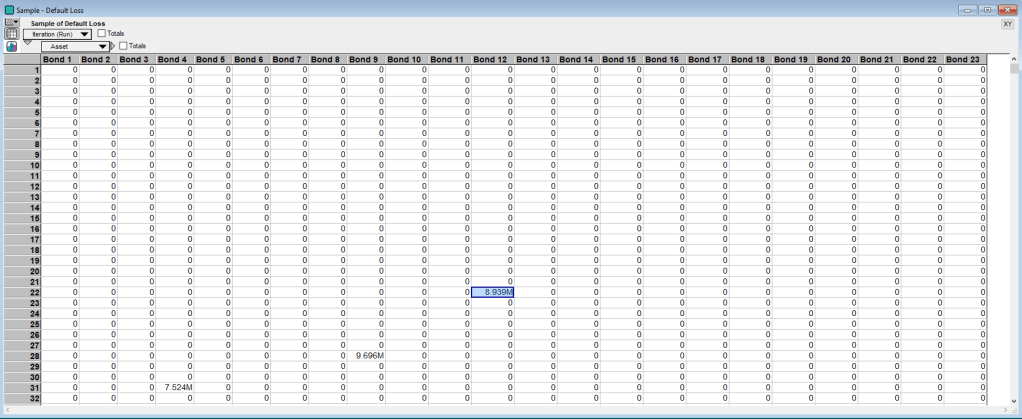
The Asset Recovery Rate then maps the simulated industry and seniority level recovery rates to the specific assets in the portfolio. The Asset Default node is an indicator variable of when an asset migrates to the default state. This node is calculated during the migration analysis. Combining this information, along with the initial dirty prices of each bond and their exposures, gives us the last node on the right, Default Loss. Default Loss is the simulated losses on default. Below is the sampling view of Default Loss and, as expected, default is relatively rare with the first event occurring in the 22nd simulation run of the model for Bond 12.

Now that we have losses from credit migrations and losses from default, these values are added together to give the losses on each run of the model. The model then generates risk measures for the portfolio, which we turn to next.

Portfolio Metrics

As mentioned above traditional statistics like the mean and standard deviation do not provide a complete picture for a credit loss distribution. However with Monte Carlo simulation we can capture the entire distribution and thus use tail risk measures to better quantify the portfolio’s risk. I posted above the loss distribution for this portfolio of assets, but here it is again so that you don’t have to scroll up:

Below are statistics for the simulated distribution. I used 30,000 simulation runs with Median Latin Hypercube sampling.

The Expected Loss is the mean of the loss distribution. The Unexpected Loss is the standard deviation of the loss distribution. The VaR at 90% is the value at risk with a confidence level of 90 percent. The desired confidence level can be altered on the assumptions panel. The value at risk is the measure of maximum loss for a given confidence level over the risk horizon. The probability that this loss is exceeded is one minus the confidence level. So here, there is a 90 percent confidence level that the loss of $5.031M will not be exceeded over the next year. Another way to say this is that there is a 10 percent probability that the maximum loss is greater than $5.031M. VaR has traditionally been the metric that regulators look to when examining the portfolio risks of financial institutions. However VaR has come under heavy criticism since the housing market collapse of 2007-08. Shin (2012) for example argues that the extensive use VaR can destabilize the market. Additionally VaR does not quantify the magnitude of losses in the tail above itself.

The Expected Shortfall risk is one such tail risk statistic used to address these issues with VaR. Expected Shortfall is the conditional expectation of the losses beyond the VaR, i.e. it is the mean of the losses above the VaR amount. Here that value is $11.67M.

Compare the results of my simulation above with Ramaswamy (2004) listed below. He uses 500,000 Monte Carlo runs.

As can be seen the model’s simulation results are very similar to his results, which offers a degree of validation. Naturally more extensive backtesting would be needed in practice.

Conclusions & Extensions

There are numerous avenues to extend the basic model here. These include conditional migration matrices to capture the broader state of the economy, relaxing the normal distribution assumption on asset returns, assessing the model at different risk horizons, and performing asset level risk assessments such as using incremental VaR to analyze the risk contributions of individual assets in the portfolio. Just to name a few.

However this post is long enough, so I leave it to readers to see the references below to further explore credit risk analysis and portfolio construction questions.

If you have any questions, feel free to email me.

References

Altman, E., Kishore, V. (1996). Almost Everything You Wanted to Know about Recoveries on Defaulted Bonds. Financial Analysts Journal, Vol. 52, No. 6 (Nov. – Dec., 1996), pp. 57-64.

Gupton, G. (2007). CreditMetrics Technical Document. New York, NY. RiskMetrics.

Hull, J. (2018). Risk Management and Financial Institutions Fifth Edition. Hoboken, NJ. Wiley.

Luenberger, D. (1998). Investment Science. New York, NY. Oxford University Press.

Ramaswamy, S. (2004). Managing Credit Risk in Corporate Bond Portfolios: A Practitioner’s Guide. Hoboken, NJ. Wiley.

Ramaswamy, S. (2005). Simulated Credit Loss Distribution. The Journal of Portfolio Management, Summer 2005, 31 (4), pp. 91-99.

Saunders, A., Allen, L. (2010). Credit Risk Measurement in and out of the Financial Crisis, Third Edition. Hoboken, NJ. Wiley.

Trueck, S., Rachev, S. (2009). Rating Based Modeling of Credit Risk: Theory and Application of Migration Matrices. Burlington, MA. Elsevier.