Introduction

One of the questions that arises in analyzing real estate development projects is how to phase the project to minimize the project’s risks over construction periods that can last months if not years. Properly phasing, that is subdividing a project into separate self-contained stages, is an effective risk strategy as it allows the developer to adjust the size of the project and alter the rate of completion depending upon market conditions. For example, if home sales in a residential project begin to lag a project manager can suspend construction until market conditions improve. Additionally, if needed, the project can be closed out early if the market is expected to stay depressed for the foreseeable future.

The ability to suspend and restart work at future dates or abandon the project completely are decisions that add value to the project in the present. These future decisions are called real options and in many cases they should be modeled explicitly to understand the true value of a project. In a previous post I discussed the merits of real option analysis and provided an example of a copper mine where the operator has the option to suspend production or abandon the mine depending upon copper’s market price and the project’s net cash flow. A similar analysis can be used to phase a real estate project, which is the topic of this post.

To keep things (relatively) simple, I based the model below on this paper by economist Graeme Guthrie. Guthrie literally wrote the book on applied real options analysis, which I highly recommend. His paper provides a detailed discussion of the solution algorithm, so I won’t get into too much detail, check out the paper if interested. While in the previous post about real options I demonstrated a Monte Carlo solution method, here the model uses a binomial tree to solve for the real option value. Trees can be faster to solve when there is a single source of uncertainty but become difficult to solve and even intractable when there are multiple sources of uncertainty (a.k.a. “state” variables).

You can download the example model below.:

It was constructed in the excellent Analytica modeling environment, which makes working with binomial trees much easier than with a spreadsheet. You will need the free version to alter the model which you can download here. I will update this post with Julia code at some point. Julia is a great open source programming language designed at MIT with data science in mind, so check it out if you have not.

The Model

As in the paper, the setting is a permitted apartment project, which consists of several construction phases with each phase having its own capital expenditure and a number of months needed to construct the phase. The project can be delayed prior to the start of each construction phase in which case a monthly suspension cost must be paid to maintain the project as an on going concern. Lastly the project can be abandoned at the start of each construction phase, if market conditions dictate. Upon abandonment a salvage value is received that incorporates close out costs and selling the property.

Below is the user panel for the model. The default settings are the values from Guthrie’s paper but any user can adjust these inputs to add phases, change capital expenditures or make other necessary adjustments to value their own projects.

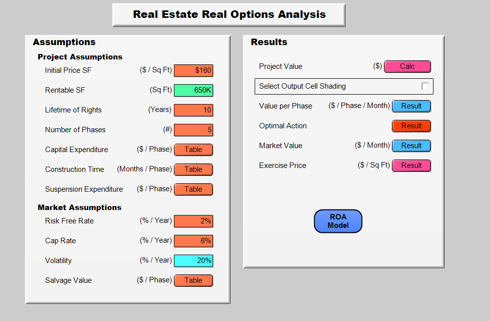
With the exception of the volatility parameter all of the inputs and assumptions are standard for real estate projects. The volatility is the standard deviation of the rate of return of the apartment’s market value. It captures our uncertainty about what that return will be in the future and therefore what the market value of the project will be in the future. Guthrie provides a nice discussion of several approaches to estimating volatility, which can be estimated from market data in several ways.

In this model the market value evolves according to a binomial probability model of asset prices without mean reversion. Mean reversion of asset prices is not present in this version of the model but can be incorporated if the empirical data dictate. (Typically mean reversion is seen in housing markets over five year periods, see Glaeser & Gyourko (2006), but whether to include mean reversion in the valuation model depends on the particular real estate market and the project’s timeline.) Observe the possible future market values of a completed apartment building in the image below:

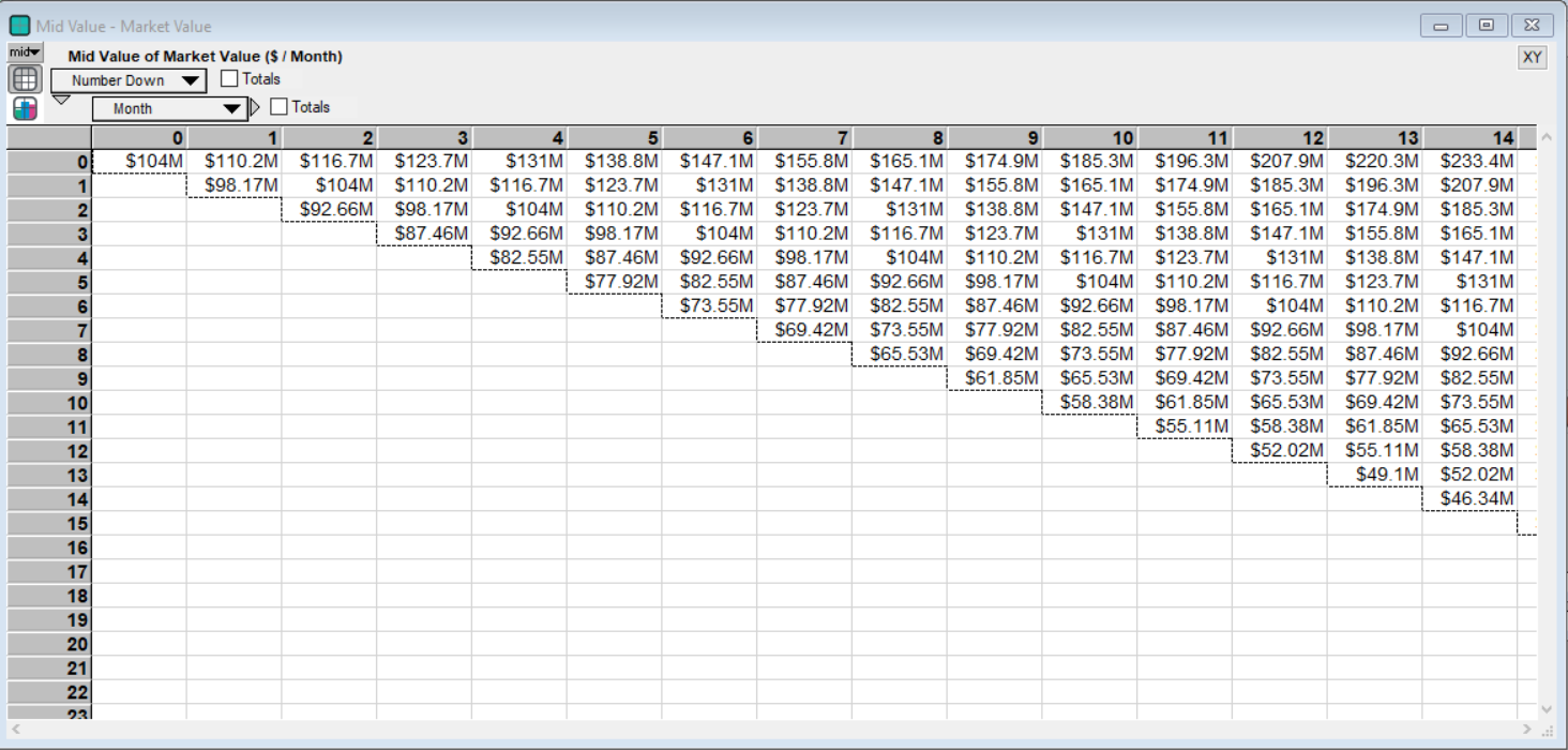
The binomial model can be thought of as a coin flip model of asset pricing. At each cell/state think of a coin being flipped where a heads means an increase in asset value, which is a move to the right in the same row, and a tails means a decrease in market value which is a move to the right but in one row down. So in Month 1 without a previous move down the project has a value of $110.2M. In the next month it can either have a value of $116.7M or it can move back to its original value of $104M if the market value decreases. The volatility parameter determines the size of the movements up and down. As you can see above by Month 14 there is a large range of values centered around the value of the project in Month 0.

Note that the values along the Number Down index (the rows) in each month are not equally likely as their individual probabilities depend on the number of paths from Month 0 that can be taken to reach a cell in the the future month. Returning to the coin flip analogy, for the apartment building’s value to be in the first row at Month 14 with a value of $233.4M there is only one path able to reach this state by “flipping” 14 heads consecutively. The event of flipping 14 heads (asset up moves) with no tails (asset down moves) is much less likely than flipping 7 heads and 7 tails, which would put the market value back at the value today of $104M. Additionally in this model the “coin” is biased so a head, up move, only has a probability of 45.79 percent. Thus that $233.4M valuation in Month 14 is very unlikely.

Once the inputs have been entered the project can be valued. As mentioned above the detailed solution procedure is described in Guthrie’s paper. But the basic idea is to work backwards from the market value of a completed project in each state to the project value today. (A single cell per phase in the table above is a state.) Thus the project value for each state in phase 5 is derived from the market prices of a completed building and the value of the project in phase 4 is derived from the project value of phase 5. This process iterates back to the starting point at Month 0 in phase 1. See the project value in phase 5 below:

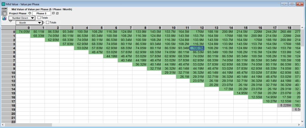
The value in each cell/state is based on the manager’s decision of whether to develop and invest in constructing that phase (green cells), delay (gray cells) or abandon the project (red cells). The action that provides the highest value is chosen. For the final construction phase, Phase 5 above, develop is often the optimal action in the early months of the project. However these states are typically unreachable because of the construction time need to complete the earlier phases. Looking at the same months for the initial phase, Phase 1, provides a different picture of the project:

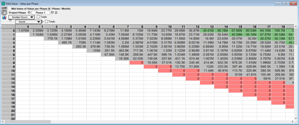
The value of the project is much lower due to including the construction costs of all five phases and discounting the market value after all phases of construction are complete. (Because we are solving for the project valuation backwards the phase 5 valuation table above only accounts for the phase 5 construction costs and not any earlier expenditures.) Another take away of the above table for Phase 1 is that it is not optimal to begin construction right away, but instead to delay until at least Month 13. Additionally the first abandonment state occurs in Month 8 if eight consecutive months of decline in project value occurs. To make the actions clearer see the following table:

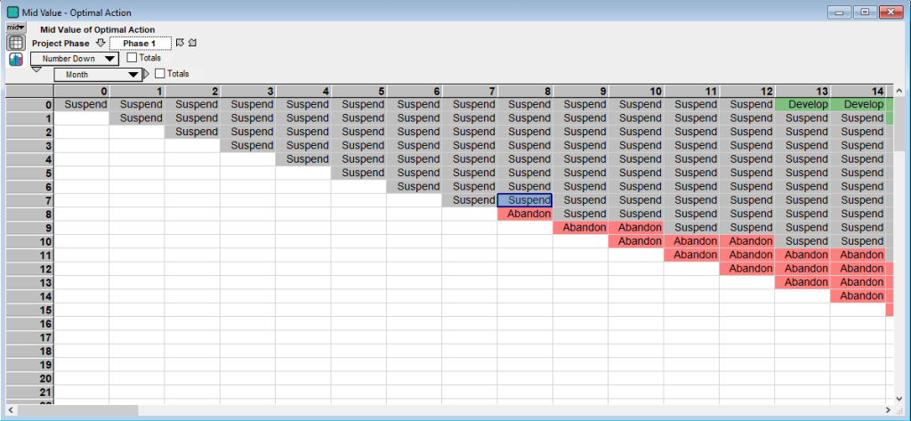
The value of the project is then the value in Phase 1 at Month 0: $1.676M. From Guthrie’s paper the table below compares the value of the real options approach to the traditional NPV approach for each phase assuming the project is in Month 0. (The “No. Stages Remaining” is the reverse of the Phase number in the model, so Phase 1 has 5 Stages Remaining):

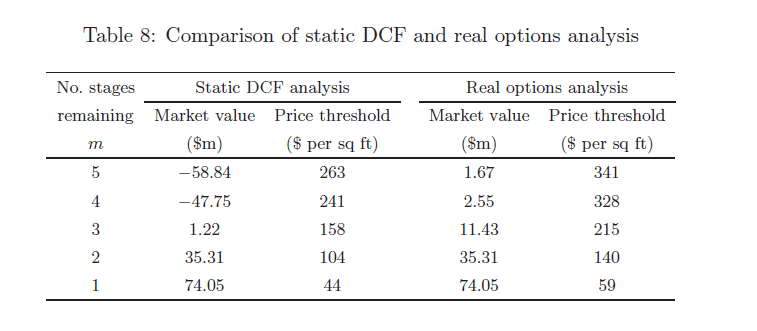
The value of the project prior to any construction in Month 0 is $-58.84M using the NPV technique and $1.676M using the real options technique. Thus we see the dramatic difference in valuation for the first three phases between the NPV and real options methods. The ability to suspend construction and delay different construction phases have a major impact on the project’s value and completely alter the decision to invest. Note that Guthrie’s paper discusses several measures of sensitivity if you are interested. I added several sensitivity measures in the model but I won’t discuss them here. Additional sensitivity tests are straightforward especially in Analytica which has the nifty WhatIf function.

Conclusion

In this post I discussed a model built to replicate a real options analysis for real estate development. One of the limitations of the binomial tree model is that it does not handle multiple sources of uncertainty well. For instance the current model assumes that construction costs are known with certainty even though in practice they are a major source of risk. In situations when it is necessary to add additional sources of uncertainty, like construction risk, the Least Squares Monte Carlo algorithm discussed in a prior post can always be used. But the tree method here still can be very effective especially as a first pass to understanding the value of different development options, as we have seen in this example.

Hopefully you found this post informative, as always email me with questions or if you have difficulty getting the model working.