Introduction

In previous posts I have demonstrated how to use Monte Carlo simulation to handle absorption risk, vacancy and occupancy dynamics, and sale price (or rental rate) risks for real estate developments and investments. In addition to those risks, real estate construction projects are notorious for being over budget and behind schedule. Therefore in this post I present a straightforward approach to modeling both the budget and the scheduling risks for a real estate construction project.

To keep things simple, the model below focuses only on generating construction draws over time and does not address project revenues or the use of decision criteria like NPV. Also, while this example is for a real estate project, the same principles can be applied to modeling costs for many different investment and project planning decisions.

I am again using the visual modeling language Analytica. To use the model, download the free version of Analytica here, and the model here: Construction Cost Blog Post Model.

If you are interested in an open source alternative to Excel or Analytica, I recommend R, Python, or Julia. An excellent introduction to Monte Carlo simulation using R applied to project level decision analysis is the book by Robert Brown, Business Case Analysis with R. R also has the ability to generate easy to use input and output panels (dashboards), which is a great feature. See the Shiny package for this capability.

Modeling Project Uncertainty

Due to the uniqueness of each project, the critical question is how to actually model the uncertainty in timing and construction cost line items. The approach taken here is to use the knowledge of a subject matter expert (e.g. a cost estimator) to encode a range of possible outcomes for each line item. Then a probability distribution can be created using the encoded ranges.  From these probability distributions thousands of different scenarios are simulated.

To this end, the model here uses a three point estimate for each construction cost line item and for the project duration (in months).  From each three point estimate a distribution is created and thousands of different scenarios are drawn.  The individual line item simulations are then combined into thousands of different S-curves, where each curve represents the cumulative construction cost over time. (See this article for the basics of S-curves in project management.)

From each S-curve a draw schedule is then easily derived since each draw is simply the incremental increase of the S-curve in that period. The simulated draw schedules can then be used in a financial model to evaluate a project’s return distribution and the investment decision.

This may sound complicated. But the actual model is quite simple once you examine the visual diagram and equations in Analytica. Model transparency is a major reason why I use Analytica for the majority of my modeling.

Note that the model and this blog post don’t get into the specifics of actually encoding a subject matter expert’s knowledge into a range of outcomes. For a deeper discussion on probability elicitation from subject matter experts see the book by Brown mentioned above. Additionally see the discussion in chapter 12 of the free PDF book Decision Analysis for the Professional by Celona and McNamee. Lastly if you are really interested in expert probability elicitation see O’Hagan et al‘s Uncertain Judgements: Eliciting Experts’ Probabilities.

The Construction Cost Model

The model has about 50 equations in 67 nodes, so I won’t walk through all the details. Instead I will describe the input assumptions and the model’s output. The ultimate goal of this type of model is to produce construction draw schedules that can be included in a broader financial model with a revenue structure.  Analytica has a nice modular structure so  embedding this model into a more complete financial model is very easy. Additionally if you want to use the output of this model with Excel, my recommendation would be to focus on the probability bands output that I will talk about below.  The probability bands give you a range of 5 different draw schedules that can then be easily integrated into your Excel model by simply cutting and pasting the schedules from Analytica to Excel.

Model Assumptions & Inputs

The default setup for this construction cost model is based on a 10 unit stick-built townhouse residential development where each unit has about 2,500 square feet of living space.  This type of infill development is currently popular in the surrounding towns of Boston, MA. Naturally the default numbers are meant to be illustrative only.  Readers can change the assumptions and inputs as I describe in this section.

Below is the User Assumptions panel where the primary assumptions are entered into the model.

The first input of interest is Cost Estimate, which is the table containing the three point estimates encoded from the cost estimator for each construction line item.  See below:

On the vertical index (axis) the line items are separated into three different cost categories, namely site costs, hard costs, and soft costs.  To add or remove line items from these categories simply right click and select add or delete depending upon which action you want to take.  The model will adjust automatically because of Analytica’s excellent array programming capabilities.

The input for each line item is a three point estimate for the low or p10 amount, the high or p90 amount, and the most likely or p50 amount.  Note that p10, p50, and p90 refer to the 10th percentile, 50th percentile, and 90th percentile, respectively, where a percentile is the probability of being at or below a given value. So for instance the first Hard Cost line item, Foundation / Foot / Wall, has a 10 percent chance of being $89K or less, a 50 percent chance of being $110K or less, and a 90 percent probability of being less than $135K.

The last column is the choice of distribution.  For this example there are only three options, the triangular distribution, the PERT distribution, and the metalog distribution which is called a Keelin distribution after its discoverer (who also happens to be a real estate investor).  Due to their flexibility, these three distributions are standard options when encoding information from a subject matter expert.

Triangular and PERT distributions are used when the max, min, and most likely values are known with a high degree of certainty but the shape of the true distribution is not known.  A possible drawback of the triangular distribution (although some may see it as a benefit) is that it has heavy tails, so the probability of simulation draws near the high and low estimates is more likely than in a PERT distribution. In this model, the Keelin distribution is unbounded on the high side and bounded by zero on the low side. The Keelin distribution uses the three point estimates as percentiles to generate the probability distribution.

In practice I usually prefer to use Keelin distributions due to their greater flexibility and their ability to capture very low probability extreme outliers, which is realistic for a construction project. The one caveat when using the Keelin distribution is that its algorithm may not always find a solution.  So the three point estimates will need to be adjusted, usually by only a few dollars, when this occurs. Unfortunately the error message for the Keelin distribution is not ideal as it does not refer to the specific line item (index value) for which it cannot find a solution. Instead the error message refers to the values of the three point estimate. If you do get an error, press cancel and then look carefully in the Cost Estimate table. The line item throwing the error can be deciphered and adjusted by looking at the three input values.

The next assumption to be entered is the three point estimate for the Project Time Estimate. This is the total number of months needed to complete the project and is simulated from the selected distribution.

The Project Time Estimate variable is used to create the S-curves that represent the cumulative construction costs over time from which the draw schedules are estimated. Since the focus here is on financial modeling and not project scheduling, the S-curve is approximated from a cumulative normal distribution where the project achieves 100 percent completion during the final project month. The final month being what the variable Project Time Estimate is simulating. Thus the model will have many different S curves.  Below is an example S-curve with Month on the horizontal axis and the percentage of the completed project on the vertical axis:

Whether to approximate the S-curve from a normal distribution or to use a total project schedule breakdown is really a question of project complexity. The more complex the project, the more it needs to be broken down into constituent parts for modeling purposes. However stick built residential projects are relatively straightforward, so I have found this approximation to be effective with the added benefit that it saves a lot of time.

After entering the project time estimate, the next input variable is the Cost-Time Correlation. The correlation between project completion time and total cost is an important consideration to make the model realistic, since cost overruns and correcting construction defects are invariably linked to longer completion times.  Thus, typically, the time to completion and the total project cost are positively correlated. (Although sometimes a construction manager can pay more to have his project completed sooner, but this is not usually the case.)  The correlation between total cost and completion time is a choice from a drop down menu:

The correlation statistic used here is the rank correlation, which measures ordinal association (i.e. rankings and not quantities).  The model will sort the project time estimates and the total construction costs so that they will have the correlation chosen above. A correlation of 0.7, since it is positive, means that longer completion times will be associated with higher total costs.

Some analysts argue against using correlation statistics and instead favor modeling interdependencies between uncertain variables through other means, such as using explicit formulas or conditioned probability elicitations.  See the Handbook of Decision Analysis page 243 for a discussion.  However for stick built residential projects historical estimates between time and cost can be used to generate accurate correlation coefficients.  So here I am deviating from what some analysts consider best practice. (Although naturally there is debate and other cost estimators do use correlations freely, see Hollman’s Project Risk Quantification book).

Results

Since this model only includes the cost side of a real estate project we cannot look at typical investment decision criteria like the NPV or the IRR.  So instead let’s just look at some tables and charts.

Project Cost Results

After the assumptions are entered, the model will simulate each line item drawing a new value for each run of the model.  Thus for the Site Cost line items the model draws the following values for the first 20 runs of the simulation:

 

The distributions (densities) for each of the site cost items generated from the three point estimates and their selected distribution have the following shapes:

 

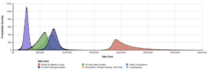
Similar charts for the Hard Cost and Soft Cost line items are on the results panel in the model.  For each run of the model, the individual line items are added together to give a total construction cost. Across all runs of the model there is a distribution for the total construction cost which looks like the following:

The total cost distribution has a long tail of low probability but high cost events which is consistent with both personal experience and related research in construction cost modeling. Additionally when we compare this distribution to the most likely cost estimate (50th percentile) of $4.35MM (= sum of the middle column of the cost estimate table above plus the construction management fee) we discover that there is about a 64 percent chance that the actual cost will be greater than this middle value. Thus this model is capturing more of the risk inherent in a construction project than a simple point estimate of the construction cost.

The cumulative probability distribution chart, below, is also very useful. For example there is about a 60 percent chance of having a construction cost below $4.5MM and a 40 percent chance of having a construction cost above that value:

Project Completion Time Results

The next result is the from the Project Time Estimate variable which is simulating the completion month.  Below is the histogram of completion months:

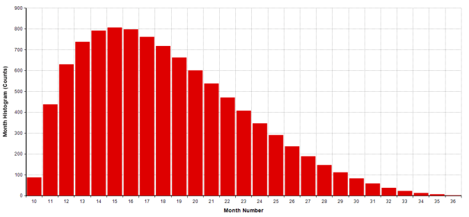The horizontal axis is the completion month and the vertical axis is the count of the number of simulation runs that have that month number as the completion month.

 

Time & Cost Results

After combining the cost simulations and the time to completion simulation the model will generate the S-curves.  Below is a chart of the first 500 runs of the model out of 10,000 total runs.

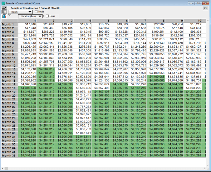
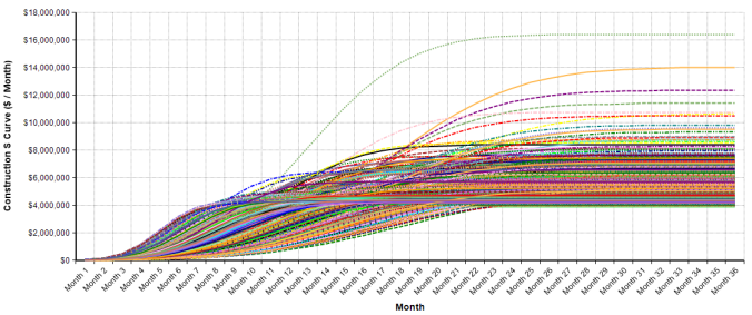Most of the S curves become horizontal before the last month because they have achieved 100 percent completion status. In tabular form, below are the S curves for the first ten runs of the model. The cells in green denote that construction is complete for that run of the simulation:

As mentioned above, from these S curves the construction draws are derived. Each monthly draw amount is simply the difference between the S-curve in that month and the S-curve value of the prior month, i.e. the draw is the incremental increase in the completion curve.

Note the large variability in construction draws. For easier viewing, below is a chart of ten randomly chosen construction draws from the model:

The final chart to look at is the probability bands (percentile ranges) for the construction draws:

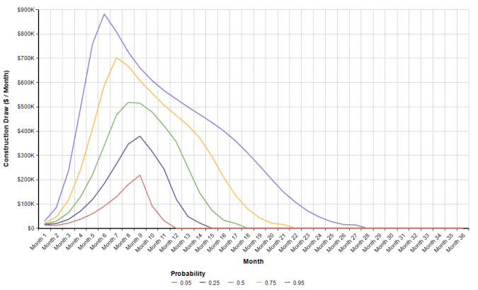
This chart shows the probability of being at each line or below.  Thus the top line shows that for each month there is a probability of 95 percent that the construction draws in that month are below this line.  Additionally this means that 90 percent of all construction draws are between the top and the bottom lines for each month. The draws can also be viewed in a table (which can be cut and pasted into an Excel model):

Conclusions & Extensions

This post demonstrated one method (among many) of generating thousands of draw schedules that can be used for the quantitative evaluation of a real estate construction project. Some of the issues that this model ignores are scheduling dependencies between individual line items and cost correlations.

As mentioned above whether a finer analysis at the cost schedule level is needed really depends upon the project at hand and where the analysis team is in terms of evaluating a project. Certainly a full project schedule for an initial evaluation is overkill. Time is of course an unreplenishable resource, so it is best not to over model early in the project evaluation process.

The other major issue that the model ignores is correlations between individual line items. For basic residential real estate I have not found much advantage in worrying about inter-cost correlations. But for more complex projects, your simulation will not be meaningful if these correlations are not considered.

As always, if you have any questions or comments, drop me a line via email.