Introduction

Real estate prices, whether they are housing prices, land prices, rental rates, or construction costs, evolve continuously through time. Traditionally real estate analysts have not directly modeled this dynamic process of price evolution. Instead they have relied on simple heuristics to handle future uncertainty, such as assuming a constant growth rate for the variable in question. Risk analysis has then been performed with a three pronged sensitivity (parametric) analysis.  While sensitivity analysis is very important in any risk analysis, it is best to complement it with additional techniques. Other areas of applied finance, such as fixed income and oil and gas exploration, have turned to more powerful simulation methods based on stochastic processes to quantify uncertainties that change over time.

The example presented below adopts a standard stochastic process to demonstrate a simulation based approach to risk quantification for a simple real estate development. This method is not meant to replace parametric approaches, but to complement them. When confronted with uncertainty and the potential for large losses, we must use all available tools to fully understand the risks, rewards, and our willingness to bear those risks. The key advantage of stochastic modeling is that it allows the analyst to focus on distributions, i.e. ranges of outcomes and their probabilities, instead of simple point estimates.

I have constructed the model in Analytica because it comes prepackaged with a fast and furious Monte Carlo engine combined with a remarkably simple syntax. Feel free to edit and run the model with Analytica’s free version. The example model can be downloaded here: Stochastic House Prices.

If you would like to perform a similar analysis in VBA then the book by Back (2005) is a great resource for both code and explanations of the mathematical finance. If you are using R, the best resource for Monte Carlo simulation applied to investment analysis is Brown (2018). (References made in the post are listed at the end with links when available.) For Python there are numerous free references on the web, so I leave you to Google. (In general Quant Econ is great as a Python primer, although it is more focused on economics than finance.)

A Simple Example

Consider a developer who must decide whether to purchase a parcel of land that can be subdivided into five single family house lots.  The project would be phased, so that the developer would build and sell each home one at a time.  Assume that there is no uncertainty over the construction costs, purchase price, draw schedule with a simple straight line draw, sale date, and all other expenses and costs. The only source of risk in this example is from the sale price, which changes over time. Additionally, to keep things simple, there is no option to suspend construction even if home prices fall below construction costs. (For a real options model that incorporates a suspension option and that can be adapted to real estate see this post.)

The assumptions used for the relevant inputs are in the panel below:

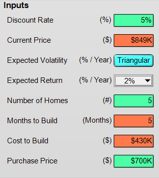
The Discount Rate will be used to assess the net present value of the project, as we will see below.   The Current Price is simply the price today of comparable housing units. This value will serve as the base price from which future prices evolve. The Expected Return is the annual rate of return for home prices, i.e., the growth rate. The Expected Volatility is the annual standard deviation of the rate of return.  Together these two inputs are the core parameters of the stochastic process that is used to simulate the housing prices over time.  They will be discussed in more detail below. The only other variable that needs explanation is the Cost to Build. The cost to build includes all site, soft, and hard costs for the construction of each unit.

With the above assumptions, the construction cost side of this example is straight forward because there is no uncertainty for these variables.  But to get a sense of how the model works, below is the construction cost draw schedule for each house:

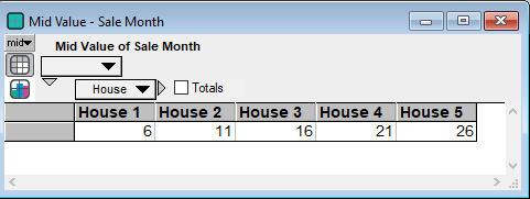
Sales occur in the month directly following the last construction draw month for a home. So the sales month is the following for each house:

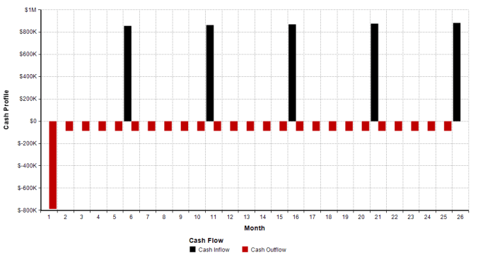
The overall cash profile of inflows and outflows is in the following chart. Note I am only taking the mean (expected value) of the sale prices, which are the cash inflows.  As we will see in the next section the cash inflows possess substantial variation in their realizations. (A realization is a single run of the simulation.)  The large initial cash outflow is the purchase of the property plus the first construction draw for the first home.

Modeling Home Prices

Due to the ever changing nature of employment, population, new construction, and obsolescence, the supply and demand of new homes is constantly changing . While this uncertainty may appear formidable at first, fortunately the brilliance of such men as Louis Bachelier, Albert Einstein, and Norbert Wiener have come to our rescue.  Building on their ideas, later researchers have applied stochastic processes with great success (and several notable failures) throughout finance.  Each day large financial institutions, hedge funds, and the finance teams at major companies use these methods to manage and understand their risks. However, outside of several of the more quantitatively orientated mortgage funds and bank departments, these methods have yet to become day to day practice in real estate firms. (For a mortgage investor’s perspective to probabilistic modeling see Schultz (2016).) While probability models are not fool proof, as the last recession made clear, they are a tremendous improvement over traditional real estate modeling approaches.

The stochastic process that we will use to model our price risk is geometric Brownian motion (GBM).  In the quantitative finance literature there are many good references discussing this process, my personal favorites are Černý (2009) and Luenberger (1998). This process is standard for many financial applications as it disallows negative values but allows for smooth fluctuations in prices. GBM is frequently used in the mortgage backed securities literature to model home prices, see Downing et al (2005). However, this process does not have a mean reversion (MR) component. If mean reversion is a concern then an alternative process to use is the Ornstein-Uhlenbeck process, see Černý (2009) for a discussion. As Glaeser and Gyourko (2007) document mean reversion typically becomes noticeable in real estate data around the 5 year mark. So if a project is expected to last longer than 5 years, using a mean reversion process may be better for investment modeling purposes.

Now there are two methods to simulate GBM that while not exactly identical do not make much of a difference in practice, see Luenberger (1998) for a discussion. For our purposes, the GBM equation that describes the evolution of home prices from one month to the next is the following:

where is the house price in period t,  is the expected annual rate of return, is the time step, is the standard deviation of return, called the volatility, and is a standard normal random variable with a mean of 0 and a variance of 1. The time step here is equal to because the parameters and are annual rates. Thus we need to adjust them to account for monthly price movements.

The two parameters that need to be estimated are the expected annual rate of return, , and the volatility, . The rate of return is the expected price appreciation for the product type in the relevant market area. One can infer this value from both recent historical data and from forecasting supply and demand.  The volatility is a little trickier. As discussed in Guthrie (2009) there are three common approaches to estimating volatility in real estate markets. The first uses an aggregrated real estate price index like the Case-Shiller Index or the FHFA index. Another approach is to use REITs as a proxy for real estate volatility. Lastly an implied volatility approach can be taken.

However for a specific project aggregated real estate price indexes are of limited use because of their aggregation. Wallace (2011) argues that these indexes were a contributing factor in the 2008 recession because aggregation inherently biases volatility downward. The second approach, using REITs as a proxy for real estate volatility, has the same problem as aggregated price indexes. REITs are typically diversified portfolios of assets. This diversification tends to reduce the estimated volatility below that of a single asset.

Thus for commercial and multifamily projects some analysts have adopted the “implied volatility” approach of Downing et al (2008). Implied volatility requires a mortgage valuation model, such as presented in Schultz (2016).  The implied volatility is then the volatility that equates the model’s predicted price (e.g. mortgage value) to the actual observed price.  This is the same method used to calculate an ordinary European call option’s implied volatility via the Black-Scholes option pricing model. The mathematical form of the pricing model being the obvious difference.  Interestingly, as Taylor (2004) documents, implied volatility in other areas of finance has a better forecasting record than estimating volatility from historical data.  See Back (2005) for a very readable discussion of volatility estimation, especially time changing volatilities. For a slightly more advanced reference see Taylor (2004).

Using implied volatility Downing et al (2008) find an average volatility of about 20 percent for a single multifamily project. This seems much more reasonable than the 8 percent volatility from the national CPPI index and the 10 percent volatility number estimated from historical REIT data.

From a decision analysis perspective, since the rate of return and volatility are unknowns, then modeling them as probability distributions is one solution to this conundrum.  Another approach is to apply sensitivity analysis to these variables.  From the sensitivity analysis we can then observe how the NPV distribution (our return criterion) changes with a change in the parameter’s value.

For this example, the model is set to perform sensitivity/parametric analysis on the expected rate of return and probabilistic analysis for the volatility. (Of course a complete model can combine the two types of analysis, but that will take us too far afield here.) The model’s expected rate of return can be set to 2 percent, 4 percent, 6 percent, or all of those values at once. However to keep this post relatively concise the results below will be for the 2 percent case unless stated otherwise.

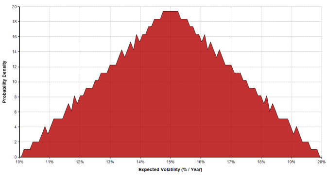
The volatility is modeled with a triangular distribution having a low value of 10 percent, a mid value of 15 percent, and a high value of 20 percent.  The triangular distribution is often used in cases where we don’t have extensive knowledge about the true distribution, but we do have a three point estimate of the variables range. The graph of the volatility’s density function is the following:

 

For each run of the simulation a value for the volatility is selected from the above distribution based on the probability of it occurring. Below are the volatilities for the first ten runs of the model:

Results

Home Prices

The first set of results to examine are the different realizations of the home prices over time.  In the model this variable is titled Price Process. Below are 500 runs of the simulation plotted on the same graph:

 

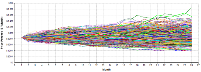
Immediately we see that the variance of price grows with time. This dispersion growth captures the reality that the further out into the future the project extends, the more uncertain we will be about the sale price. Another immediate observation is that for each sale month there is a distribution of prices, with many possible prices below the starting value and many above the starting value.

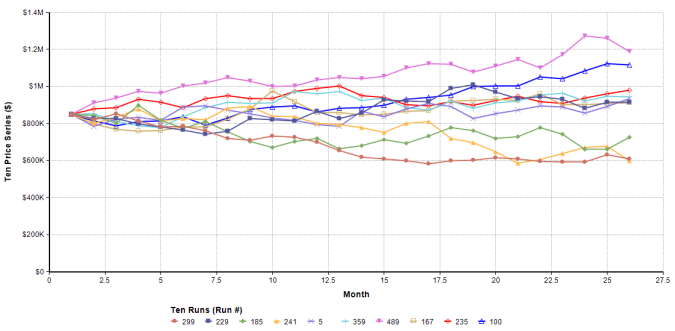
Now 500 realizations in one chart makes it is difficult to see the randomness of each price path. So below is a random sample of ten such price series where each run represents a single possible future for prices:

 

Another graph that is useful to understand the range of outcomes is to view the probability percentiles.  Recall that each percentile is the probability of being at or below each price. The 90 percent confidence interval is the range of values between the top (95th percentile) and bottom (5th percentile) lines :

 

Numerically the percentiles for each home on their sale date are below:

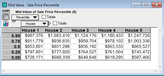
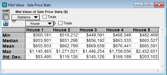
Clearly we see a wide range of sale prices that grows even wider with time and therefore increased uncertainty. Additionally it may help to look at some other statistics. Note that the 50th percentile is the median, hence they have the same value:

Return Metric – NPV

Now to determine the value of a project we need a single number called a return metric.  This example uses the net present value as its return criterion. Usually when working with simulation based models the NPV is a superior choice compared to the ever popular IRR. The reason is that simulation exacerbates the limitations and drawbacks of the IRR, such as the problem of multiple IRRs for a single cash flow stream.

The first graph to exam is the density of the NPV as this gives a sense of the range of possible outcomes.

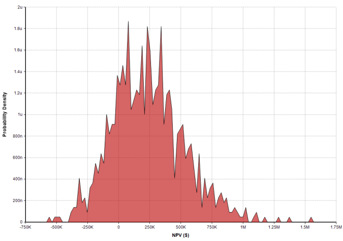
Immediately we see the possibility of having an NPV as low as $-500K and as high as $1.5M.  The bulk of the distribution appears to be between $-250K and $750K. In fact there is about a 92 percent chance of being between those two values.

To calculate probabilities, which will act as our actual decision rule, the cumulative distribution is used.  The values on the vertical axis represent the probability that the NPV will be equal or less than the corresponding values on the horizontal axis. Click on the chart for a popup balloon do give the numeric estimate:

 

Thus in the 2 percent expected rate of return case, there is about a 20 percent chance that the project will have a negative NPV.  This means that there is an 80 percent chance of the project having a positive NPV. (These values can be computed directly in Analytica with the Probability function.)

Here we will perform some sensitivity analysis on the expected rate of return. Below is the cumulative distribution for three different expected rate of return cases:

As stated above the probability that the NPV is negative for the 2 percent rate of return is 20 percent. This probability falls to 15 percent and 13 percent for the 4 percent and 6 percent home price appreciation rates, respectively.

Ultimately the decision to pursue this project comes down to risk preferences and whether the probability of achieving a positive NPV is worth the risk.  This is a subjective choice that ideally requires modeling the decision maker’s utility function. That is fodder for another time.  But if interested, see the book by Clemen and Reilly (2013) for a systematic approach to model a decision maker’s risk profile and utility function.

Conclusion

In this post I presented a simple stochastic process to model our uncertainty about future home sale prices and the resultant distribution of NPVs. Of course in a complete model we must consider all sources of uncertainty, such as the construction cost uncertainty and absorption risk. The absorption risk is the probability of a sale (or the number of sales) in each sale period.  In an earlier post I demonstrated one method for handling project absorption risk. And for construction cost uncertainty see this post.

Together these models will help an investor better understand the risks and rewards that they face.

As always, email me if you have an questions.

References

1. Back, K. (2005). A Course in Derivatives Securities. Springer. (Amazon)
2. Brown, R. (2018). Business Case Analysis with R: Simulation Tutorials to Support Complex Business Decisions. Apress. (Amazon)
3. Clemen, R. Reilly, T. (2013). Making Hard Decisions. (3rd Edition). Cengage Learning. (Amazon)
4. Černý, A. (2009). Mathematical Techniques in Finance: Tools for Incomplete Markets. 2nd Edition. Princeton University Press. (Amazon)
5. Downing, C. Stanton, R. Wallace, N. (2008). Volatility, Mortgage Default, and CMBS subordination. Unpublished Manuscript, U.C. Berkeley. (PDF)

6. Downing, C. Stanton, R. Wallace, N. (2005). An Empirical Test of a Two‐Factor Mortgage Valuation Model: How Much Do House Prices Matter? Real Estate Economics (33) 4, 681-710. (Link)

7. Glaeser, E. Gyourko, J. (2007). Housing Dynamics. Harvard Discussion Paper 2137. (Link)
8. Guthrie, G. (2009). Evaluating Real Estate Development Using Real Options Analysis. (PDF)
9. Luenberger, D. G. (1997). Investment Science. (1st Edition). Oxford University Press. (Amazon)
10. Schultz, G. (2016). Investing in Mortgage-Backed and Asset-Backed Securities. Wiley. (Amazon)
11. Taylor, S. (2005). Asset Price Dynamics, Volatility, and Prediction. Princeton University Press. (Amazon)
12. Wallace, N. (2011). Real Estate Price Measurement and Stability Crises. Fisher Center Working Papers. (PDF)