Introduction  

The Joint Venture distribution structure, aka the Waterfall, determines the allocation of profits among the equity investors and managers in a real estate project or transaction.  Typically as a project achieves different return requirements, called hurdles, this allocation of profits between the parties changes.  For this reason the Waterfall is often considered the most complex portion of a real estate model.  Its name derives from the flow of cash filling each hurdle level or “pool” and then cascading into the next level.

In this post I will briefly review some of the theory behind why Waterfall distributions exist.  Additionally I will walk through how to use a standalone Waterfall distribution model that I created.  This model can be used with your Excel or Argus cash flow models simply by copying and pasting in the appropriate investment and profit cash flows. The only other requirement to use this app is that you download the free version of Analytica. You can download the Waterfall model here: JV Waterfall.

The advantage of using the model below instead of Excel is that Analytica embraces the array programming paradigm.  Widely used in data science programming environments, array programming makes manipulating multi-dimensional objects straightforward and easy. This is relevant for us because we will want to alter the Waterfall’s dimensions, e.g. the number of hurdles or scenarios, and then allow the logic of the model to adjust for these new parameter values with no additional effort on our part.  Analytica also integrates very easily with Excel.  Excellent open source alternatives to Analytica include R and Python with NumPy.

Why Waterfall Distribution Structures Exist

In practice Waterfalls occur in myriad forms with each having its own unique features.  But at its core the Waterfall comes down to one word, incentives. Because managers can use effort and make decisions that are not perfectly observable, and may not align with the goals of limited partners, real estate funds and JVs embody what economists call the principal-agent problem. A classic solution to this problem is to align the incentives of the principals and agents through a contract that possesses a convex payoff for the agent based upon an observable outcome. The simplest example of a convex payoff is the payoff structure of purchasing a call option, see this diagram. The basic idea is that increasing the payoff to the agent without increasing the downside risk will help motivate the agent to act in accordance with the principal’s goals.

In real estate, the Waterfall structure exhibits this convex payoff for the managers, who are the agents in this principal-agent problem. As with a call option, the Waterfall’s promote allows the manager to increase their return without increasing their downside risk. At least in theory, this will help to align the manager’s goals with those of the limited partner’s. The observable outcome used for the Waterfall is typically an equity multiple or a rate of return.

The literature on principal agent problems is very extensive, see Google Scholar for more. However as discussed by Palgiari [3]  (references are at the end of the post), in practice the Waterfall’s payoff structure can alter the manager’s behavior in undesirable ways.  Specifically, when a manager is close to a return hurdle, they may take riskier actions to try and hit the hurdle.  Additionally, when the manager has already achieved a hurdle then they may become unnecessarily risk averse.  Palgiari suggests mitigating these issues by lowering the hurdle rates and the residual distribution. The scenario analysis feature of the model below can be used to explore these issues.

A Waterfall App

Now let’s look at a waterfall model that can be used alongside your Excel or Argus cash flow models.  Following the terminology set forth in Schneiderman and Atlshuler [4], the model presented below is an investment centric waterfall model.  This means that the cash accruals for each hurdle tier are calculated from the total invested equity and not just the limited partner’s equity.  This method can favor operating partners and is more common in smaller real estate projects. Institutional investors will typically negotiate investor centric waterfalls, which focuses only on the return to the investor or Limited Partner as the determinant for when a hurdle has been achieved.  Adjusting the model for the investor centric case is fairly straightforward, as the model’s logic does not change significantly.

Following Carey [2] this model will only include Hard hurdles and not Soft Hurdles.  Soft hurdles, which include provisions for look-backs and catch-ups, are extensions of the basic model presented here.  A hard hurdle acts as a deductible that once achieved will be applied to the profits for the next hurdle level or the residual level.  Soft hurdles are typically contingent upon the performance of the asset or investment.  See Carey’s article for further discussion.

Some other final notes on terminology: a Tier in this model is either a Hurdle or the Residual.  The residual is the remaining cash after the last hurdle rate has been achieved.  Since the residual and the hurdles are calculated differently, I prefer to label them differently.  But each hurdle and the residual count as separate tiers.  Many modelers will often call the residual a hurdle even though there is no return criterion being “hurdled”. Additionally “partner” is a generic term used throughout the model that is not meant to specify any legal structure.

Using the Model

Now I will walk through an example demonstrating how to use this model. When you open the model the inputs and output forms are in the respective modules User Inputs and Return Metrics:

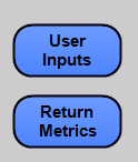
Opening the above modules and placing them side by side is an easy way to input your assumptions and return your results:

Let’s walk through the left panel, the assumptions and inputs.  The first thing to do is to enter the dates that index your cash flows.  The button Reset Dates will clear any previously entered and saved dates making it easier for new dates to be directly copied and pasted from Argus or Excel.  Just click “List” to open the following window:

The dates should be ordered from earliest to latest, but there need be no set timing schedule between each date.  The model calculates a daily accrual rate based on the number of days between each date. So it is robust to entering monthly, daily, or annual date steps and any combination thereof.  Note that you are “limited” to 32,000 values for a single index in the free version of Analytica. So in this case you can have up to 32,000 dates, which should be plenty for your model.

The next items to enter are the number of scenarios and the partner names:

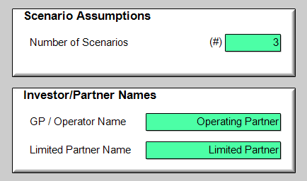
The number of scenarios is the number of different waterfall structures that we would like to compare. This is an example of the array programming paradigm mentioned above. Analytica will recalculate the model for each scenario automatically.  As with the dates, the number of possible scenarios is 32,000, far more than you will need.  After entering your scenarios, in this case 3, type in the different names for each partner. The names will appear on the final summary statement of cash flows and return metrics.

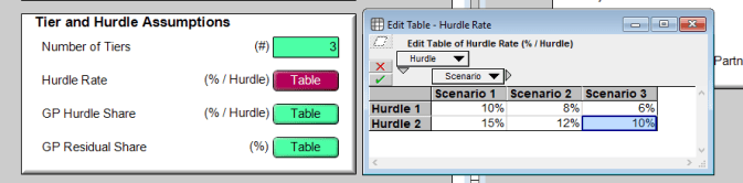
Now onto the Tier and Hurdle Assumptions.  Once you enter the Number of Tiers (the number of hurdles plus one for the residual) the next two variables Hurdle Rate and GP Hurdle Share will have their table’s columns and rows adjusted automatically.  For example, with 3 tiers (2 Hurdles + the residual) and 3 scenarios the input table for Hurdle Rate is:

Similar tables open for the GP Hurdle Share and GP Residual Share:

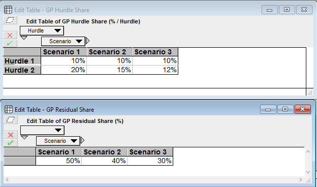
The GP Hurdle Share is the percentage of each hurdle’s cash distribution going to the general partner / operating partner. The GP Residual Share is the percentage of the residual going to the general partner. The limited partner’s share is calculated from these tables.

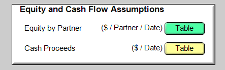
The last two input tables are for the equity investment made by the partners, Equity by Partner, and the cash profit or proceeds generated by the project, Cash Proceeds:

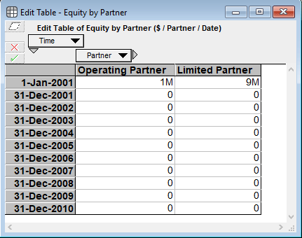
Opening Equity by Partner displays the following table:

and the Cash Proceeds table is:

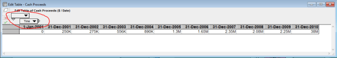
While either negative or positive values can be entered into the Equity by Partner table, only positive values are to be entered into the Cash Proceeds table since these cash flows are profits to the partners. All cash flows entered into the Equity by Partner variable are considered invested cash.  Some Excel models will have this as a positive input and others as a negative input, so the model will handle either situation.

Also note the orientations of the two tables above.  To copy and paste from Excel or Argus, the Analytica tables must have the same orientation as the Excel or Argus data.  In the above table I circled in red the drop down menus that allow easy pivoting of a table’s orientation. Select the correct orientation, and then paste in your cash flows. Note that table orientation does not matter for lists, such as when pasting into the Enter Dates variable above.

Return Summary

Let’s now look at the model outputs. Referring back to the first figure, the opened module on the right displays the return metrics panel:

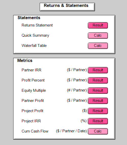
The three metrics at the top, Return Summary, Quick Summary, and Waterfall Table are all result tables.  Click the buttons to open them.  The list of metrics below these three are all included in Return Summary and Quick Summary (except cumulative cash flow).  I broke them out individually in case a user is interested in focusing on a specific metric.

The Returns Summary is the primary table for the return metrics and cash flows.  See below, and note how it has a Scenario index at the top with arrows next to it to change the table to the different scenarios:

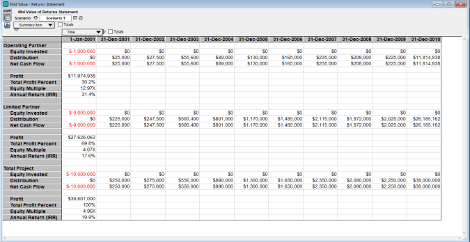
The table above shows the investment cash flows, distribution cash flows, and several return metrics for each partner and the project as a whole.  The entire table can be selected by clicking the cell in the upper left corner above “Operating Partner”.  This allows the user to copy and paste it into Excel.

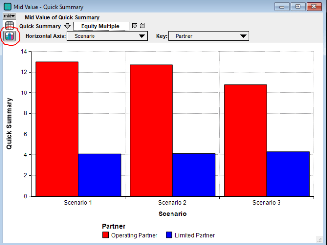
The next button in the Return Metrics module is the Quick Summary, which makes it easier to compare the profit, profit percent, equity multiple, and IRR (which is really the XIRR) for each partner and each scenario. An example for the equity multiple is below:

Additionally, another advantage of Analytica is it automatically generates a graphical display.  For the Equity Multiple click the button circled in red to see the graph below:

Lastly the Waterfall Table button returns the Waterfall for each scenario and hurdle level:

Internals of the Model

The section above focuses only on how to use the model from the assumptions and results panels.  I won’t go through every variable as Analytica strives for referential transparency and uses a simple syntax to define variables. If you are interested in understanding how this model works then simply work through the Analytica tutorial. After doing so, the definitions in this model will be easily understood.

But since I have discussed array programming in several places above, a representative example is warranted. Below is the main influence diagram for the model. This portion of the model includes the calculation of the cash accruals and distributions in the Waterfall.

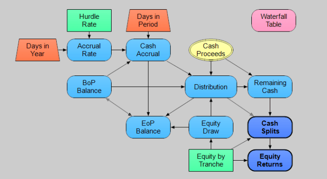
Let’s focus on the variable Cash Accrual in the influence diagram above. Upon evaluating Cash Accrual the results table is:

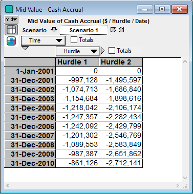
The most important element to observe in the table is that it has three different indexes, Time, Scenario, and Hurdle. Note that the result table of Cash Accrual has a total of 66 cells (11 Time steps, 3 Scenarios, and 2 Hurdles, 66 = 11 x 3 x 2). The number of cells will adjust automatically when inputs are changed for each of the three indexes. To see how each cell is calculated double click the Cash Accrual node to open its Object Window:

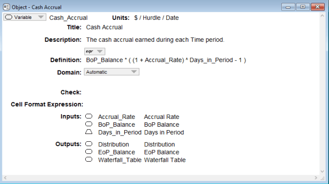
The definition is:

BoP_Balance * ( (1 + Accrual_Rate) ^ Days_in_Period – 1 )

Like most array programming languages, Analytica’s syntax is designed to try and represent each definition as a simple mathematical equation, just as if you were working the problem with paper and pencil. In English, Cash Accrual is the beginning of period balance multiplied by the accrual rate, a daily rate of return, raised to the number of days in each time period, and subtracted by one so that the BoP Balance is multiplied by the appropriate rate for the given time period. Below are the results tables for each of the inputs variables, BoP Balance, Accrual Rate, and Days in Period:

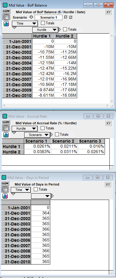
What happens during the calculation of Cash Accrual is that Analytica (and other array programming languages) will match the index values across each variable, and then execute the definition on the different variables’ values at that index address.  So for instance to calculate the value of Cash Accrual at Hurdle 2, Scenario 1 for the Time of 31-Dec-2001, the definition evaluates -10M * ((1 + 0.0383%) ^ 364 – 1) which is about -1,495,597.   (Note there is some round off error as the accrual rate is more exact in Analytica than what I typed.)  Also observe that Accrual Rate and Days in Period each have fewer indexes than BoP Balance and Accrual Cash.  When this occurs the evaluation engine will extend the same values along the indexes that they don’t possess during calculation. This is called array abstraction and greatly eases model construction.

Now every array programming language has unique features, advantages and disadvantages, and most are primarily used in engineering settings. But these languages allow us to build simple and extensible applications like the Waterfall model presented above. I expect more and more business applications to begin taking advantage of these languages.  As always if you have any questions feel free to email me.

 

Some References

Below I have added some references on promote and fee structures for those interested in reading more on the topic.  Enjoy!

1. Carey, S. (2013). Real Estate JV Promote Calculations: Basic Concepts and Issues. Real Estate Finance Journal. Summer. (pdf)
2. Carey, S. (2008). Real Estate JV Promote Calculations: Catching Up With Soft Hurdles. Real Estate Finance Journal. Spring. (pdf)
3. Pagliari, J. (2015). Principal/Agent Issues in Real Estate Funds and Joint Ventures. Journal of Portfolio Management 41(6), 21-37. (pdf)
4. Scheiderman, R. and D. Altshuler. Key Considerations in Joint Venture Projects. Chapter 11 in PERE’s Real Estate Mathematics, October 2011 (pdf)