Introduction

The previous post reviewed two of the fundamental problems with the typical approach to modeling future real estate leases, namely a failure to address the uncertainties and nonlinearities embedded in the analysis. The proposed solution for these issues is to use simulation based methods.  The example model presented in the last post simulated the physical occupancy and vacancy for a multi-unit property over time.

This post will take the next step and add the monthly rental income cash flows to the model. Our goal continues to be overcoming the flaws of the traditional method for analyzing expected property cash flows, as discussed in the prior post.  However to keep this post somewhat manageable I will not discuss incorporating lease commissions, tenant improvements, and many other elements that are needed for a complete analysis. The plan is to cover the additional elements in future posts.

I will continue to use the program Analytica, since it is my favorite modeling environment. Here is the free version. The R language is also a good alternative for real estate simulation, although less user friendly.  (See this short and inexpensive book for a very nice introduction to R simulation.)  You can play with the rental model here: Stochastic Rent Model 110817. However it is for expository purposes only, so no warranties are implied of any kind.  That said, feel free to email me with any questions.

If you would like to alter the model’s assumptions, I have updated the user input and output nodes from the previous post and placed them in the modules named User_Inputs and Results.  Just open these modules to change the assumptions and view the results.  Below I have opened both of them, and placed them side by side so that you can see what they look like:

The road map for this post is the following: in the next section I will give an overview of the rent model and the additional variables added to the vacancy model from the last post.  I will then provide a breakdown of the results for the rental income.  Lastly I will walk through some of the code used to calculate the property rent over time.

Rent Model Overview

Let’s begin by examining the influence diagram  of the model to understand the dependencies on the variables of interest, Rent and Total_Rent:

The first thing to notice is the presence of two modules (the rounded rectangles with black borders) that each contain their own influence diagrams.  The module Vacancy is the model from the previous post.  It is simply inserted into the present model, something Analytica makes very easy because of its support for modular programming. The nodes In_Place_Lease_End_Month and Lease_Month are both calculated in the Vacancy module, and discussed in the prior post. But to recap, In_Place_Lease_End_Month identifies the month when the initial leases end, and Lease_Month simulates the different possible future leases for each unit on the property.  The values of Lease_Month are the month numbers for each lease, so 0 means the lease is vacant, and 5 is the fifth month of a lease.  I have made aliases, and placed them on this top level diagram to visually identify them as parent nodes for  Rent.  Their titles are italicized to indicate that they are aliases (i.e. refer to a variable elsewhere).  The originals are still in the Vacancy module.

The other module on the diagram, Market_Dynamics, contains the variables simulating the evolution of the future market rent in the eponymously named variable, Market_Rent.  Since this is a simple example, Market_Rent takes the rent from the previous year, but in the same month, and then adjusts it with an independent draw from a normal random variable.  The normal distribution used here has an annual mean of 1 percent, and an annual standard deviation of 2 percent.  To make this more concrete, below is the statistics result window view for Market_Rent.  The selected statistics displayed for unit 3 are the mean, the maximum, and the minimum over time.

During the first twelve months of the analysis period Market_Rent is the current market rate as entered by the user, so that is why there is a constant horizontal line for that time period.  The mean statistic increases in a step like fashion because the rent increases with a mean of 1 percent per calendar year.  But as argued in the previous post, we care about the dispersion of our investment returns, so it is important to get a feel for the maximum and minimum rent values over the time period, conditional on our assumptions.  As shown on the chart, even with a relatively small standard deviation of 2 percent per year, the minimum is below the rental rate at the time of acquisition, so the property is losing value in this downside scenario.  The other units have similar values but adjusted for their particular current market rent at the time of acquisition.

This approach to forecasting market rent is admittedly stylized, despite it being very close to what often occurs in practice with respect to the average annual increase in rent.  Performing a proper market analysis and incorporating uncertainty into that market analysis is a deep area that we can only dip our toes into at the moment.  In reality an investor needs to fully understand the local submarket, and the investor should complete a comprehensive market analysis to properly forecast the expected supply and demand over the analysis period.  But for this example, and to create some variance in the future market rent, I calculated it as above.  Feel free to play with the mean and standard deviation assumptions, as they are on the User Input forms discussed above. For another approach to modeling rental dynamics see this post.

The next new node in the influence diagram is In_Place_Rent.  This is an edit table where the user enters the rent for the units leased at the time of acquisition.  In this example we have the following rental assumptions:

It is important to observe on the diagram that In_Place_Lease_End_Month is a parent node to In_Place_Rent, despite In_Place_Rent being a constant node.  The reason this node has the constant shape is that the data is historical and therefore set at the start of the model.   The relationship between In_Place_Lease_End_Month and In_Place_Rent arises, not through the definition of In_Place_Rent, but through its Check Attribute.  To see this open the object window of In_Place_Rent which shows all of the activated attributes for the node:

The Check attribute has a formula that depends on In_Place_Lease_End_Month, hence the arrow from In_Place_Lease_End_Month to In_Place_Rent.  The check attribute ensures that the value of the executed definition conforms with the expression in Check.  If not, then the error message written into Check will appear.  Here the Check attribute is ensuring that the entered lease rents are zero for vacant units.  Check greatly helps in reducing user entry errors from propagating through a model.

The next node is Free_Rent.  This variable has the decision shape since the owner decides how many months of free rent to offer.  The question of where to place Free_Rent in a model is an interesting one.  Since it is a decision, the decision should be chosen to maximize NPV.  Additionally in models where the probability of a new lease is derived from a logistic regression analysis, Free_Rent may be used as an explanatory variable, since increasing the number of months rent free decreases a tenant’s total expenditure, and thus increases the probability that a unit is leased each month.  This would make Free_Rent a parent node to Lease_Probability.  However, since rental concessions can become quite complicated due to this feedback loop, I will reserve this dependency for another post.  In this model Free_Rent will serve only to determine when rental income is actually received.

The Rental Income

Now that the new nodes have been described let us turn to the results, Rent and Total_Rent.  While Total_Rent is the primary variable of interest, it is instructive to look at an individual unit’s simulated rental cash flows.  Below is the sample view for unit 3, where each column represents a run of the model, i.e. a possible future:

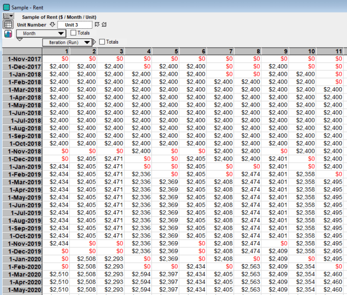
The vacant and rent free months are, obviously, in red. Although the lease terms are set to 12 months, rental income arrives in sequences of eleven months since Free_Rent is equal to 1 month.  How Rent is calculated will be discussed in the next section.

Turning to Total_Rent, which is the rent summed across every unit, the chart below is the mean value of the total rent over time:

The first thing to notice in the above chart is the oscillatory nature of the cash flows.  This is precisely what we should expect because of the transition lag between a unit becoming vacant and then being leased again at the market rate.  As noted above, on average Market_Rent is increasing steadily at 1 percent per twelve calendar months, so the oscillatory behavior is not being driven from the variance embedded in the rental market dynamics, just from the vacancy dynamics.

The jaggedness at the beginning is a result of two factors.  The first is that at the time of acquisition two units are vacant, and so their vacancies are occurring in the same month with greater frequency than occurs later in the time series, once the randomness of vacancy takes hold.  The other factor is the presence of the initial leases. I entered these leases in randomly to test the robustness of the model, so they are a bit unrealistic. Thus the lowest point in the average cash flow series occurs on 1-March-2020, the month immediately after the last of the initial leases ends.  Once the initial leases and the initial vacancies settle down the time series becomes much smoother, but still oscillatory, as is to be expected.  Even with the stylized market assumptions, this is a much more accurate representation of average rental cash flows in practice than the usually assumed constant increase.

The next chart includes both the uncertainty from the leases and the market rent.  The chart has five percentiles that denote the probability of being equal to or less than that value.  The percentiles displayed here are the 5th percentile, 25th percentile, 50th percentile (median), 75th percentile, and 90th percentile.  The percentiles also identify the probability of being between any two values, thus the future rents have a 90 percent chance of being between the top line (95th percentile) and the bottom line (5th percentile).

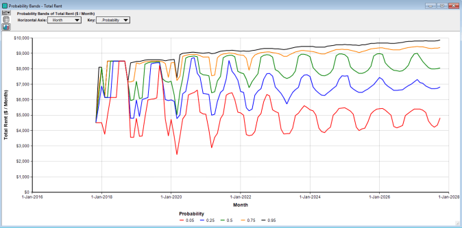
Again once the initial leases and the initial vacancies end, we see smoother behavior in the time series.  Also since this view includes the variance in the market rent, we see the large discrepancy in rents that can occur even with only a modest standard deviation of 2 percent per year for the market rent.  The table below shows that there is close to a $5,000 dollar difference between the 5th percentile and the 95th percentile in the final month.

Taking averages over the month index, the 95th percentile is on average about 81 percent greater than the 5th percentile.  Thus even with relatively simple and stable rent and lease dynamics there is a large amount of uncertainty over the rental income.

Code Snippet

The variable Rent contains the most involved code in this model, so I will walk through it here. The definition of Rent is:

Dynamic[Month](
		/* First Month */
	In_Place_Rent
	+ (Lease_Month = 1 and Free_Rent = 0) * Market_Rent,

		/* Other Months */
	If @Month <= In_Place_Lease_End_M
	Then In_Place_Rent
	Else if Lease_Month <= Free_Rent
	Then 0
	Else if Lease_Month = Free_Rent + 1
	Then Market_Rent[Month - Free_Rent]
	Else Self[Month - 1]
)

The first line initializes the dynamic function in Analytica, and sets the index over which Dynamic will step to be the Month index.  The code for the first month is

In_Place_Rent + (Lease_Month = 1 and Free_Rent = 0) * Market_Rent

The In_Place_Rent is simply the user entered rent for the initial leases. However since vacant units may become occupied in the first month of the hold period we need the additional code (Lease_Month = 1 and Free_Rent = 0), which returns a 1 or 0 depending upon whether both conditions are met or not. The first condition, Lease_Month = 1, tests for whether a vacant unit actually becomes occupied. The second condition, Free_Rent = 0, tests for whether an occupied unit pays rent in the first month. If both of these conditions are met, then (Lease_Month = 1 and Free_Rent = 0) = 1 and this is multiplied by the market rent, which returns the market rent in the first month, since In_Place_Rent would be zero in this case.  If either one of the conditions is false, then (Lease_Month = 1 and Free_Rent = 0) = 0 and no rent is received for that unit in the first month.

The code for the months after the first month is a series of conditional statements to test for the different rent conditions. The first line of code in this section, If @Month <= In_Place_Lease_End_M, tests for whether the initial leases, the leases in place prior to acquisition, are still active. If yes, then the rent for these months is the next line, Then In_Place_Rent.

If the initial leases have ended, then the next test, Else if Lease_Month <= Free_Rent, checks for whether a unit is in the Free Rent period. Additionally I have set the domain attribute of Free_Rent to be an integer with a minimum value of 0. Thus the test on this line also checks for a vacancy, since that is equivalent to Lease_Month = 0. If this test is true for either reason, then the next code line applies, Then 0, and the rent is 0 for that month.

If the Lease Month is greater than the Free Rent, then we need to assign the correct rental amount to this month. The line Else if Lease_Month = Free_Rent + 1 checks to determine that the month of the lease is the month immediately after the free rent period. If true, then the rent is equal to Market_Rent[Month - Free_Rent], the market rent at the time the leased was signed. If we are in a Lease Month after the first month with a payment then the rental amount simply equals last month’s payment, i.e Else Self[Month - 1], the rent for an occupied unit after the free rent period ends.

Wrapping Up

So now we have added the monthly rental income to the vacancy model.  As we see even modest assumptions about the vacancy and market rent dynamics can lead to significant variation in monthly rent.  Of course in a full model there are many additional factors that need to be considered, prior to making an investment recommendation or rejection.  But adding and simulating the vacancy and rental cash flows leads to a sharper and more consistent analysis between potential investments.