Introduction

This post is part of a series of posts that will demonstrate the benefits of adopting simulation as the mode of analysis for real estate investment valuation.  The focus of this post is how to conduct a lease analysis without relying on simplistic averages and blended rates that fail to properly account for uncertainty about the future property leases.  The post is structured as follows: I will first provide a brief review of how lease analysis is traditionally performed.  Then I will discuss the dual problems with this approach, namely the inability to handle uncertainty effectively and Jensen’s Inequality.  Next I will demonstrate a simulation that captures thousands of different possible future lease scenarios for a income producing property.  Lastly, I will review the important parts of the code on how to generate the simulation.

Traditional Future Lease Analysis

In real estate investment, Market Leasing Assumptions (MLA) are critical model assumptions that real estate investors make regarding the future performance of a property after the current leases expire.  These assumptions encompass a variety of future conditions that include expectations of future market rents, rent concessions (e.g. free rent), tenant improvements, leasing commissions, general economic conditions, and vacancy/occupancy rates.

The traditional approach to quantify future leases involves forecasting rental market variables, the MLAs, and then combining or “blending” these variables with the lease renewal probability, , to create a weighted average.  The logic for using these averages is that the terms of a renewed lease are usually different than the terms for a new lease.  For example the expected future property rent is given by the following formula:

where is the expected (aka “blended”) property rent, is the rent on a renewed lease, and is the forecasted market rent, if the lease is not renewed.

Likewise, the blended property lease commission, , is:

where is the lease commission for a renewed lease, is the lease commission on a new lease, and is, again, the probability of renewal.  Note that lease commissions are typically quoted in percentage terms.

Continuing in this vein the blended tenant improvements, ,  and blended months vacant, , are calculated respectively as:

where is the tenant improvement for a renewed lease, and  is the tenant improvement for a market rate lease.  The blended months vacant, , is simply the forecasted number of months vacant if the unit goes to market, , discounted by the renewal probability.

The above blended values are then entered into a pro forma model to determine the property’s investment return characteristics.  Common return metrics include the NPV and the IRR.  It is important to recognize that all of the forecasted lease variables above are functions of time, and therefore will change as economic fundamentals, like inflation and the state of the economy, change.  See Brueggeman and Fisher for a further explication of this approach with an example.

Problems with the Traditional Approach

There are two general and powerful criticisms that can be leveled at the blended rate approach above and traditional real estate modeling in general.  The first problem is that the blended rate analysis fails to adequately account for uncertainty in the variables of interest.  Any measure of uncertainty must consider both the expected value and its variance or dispersion.  This lack of dispersion in the inputs means that there is no measure of dispersion for the resulting return estimate.  It is highly unlikely, if not impossible, that the estimated returns will equal the actual returns, so having a measure of variance is an important consideration in any investment decision.

Some analysts try to evade this criticism with a tripartite scenario analysis involving a “Low” state, a “Most Likely” state, and “High” state.  But this approach fails to capture an adequate range for each variable. Additionally simple scenario analysis offers no quantification for the likelihood of any of the states occurring.  Instead, using a probability distribution for each input variable will sharpen the analysis and allow the analyst to capture a broader range of possibilities. Furthermore questions regarding independence and correlation between the input variables can be considered. How to arrive at a specific probability distribution, through statistics and elicitation from subject matter experts (for the latter see chapter 12 here), will  be considered in future posts. Here is a good reference that discusses distribution selection.

The second criticism is more technical and quite subtle, so I will just briefly summarize it here.  In practice real estate models tend to become quite complex, or in math-speak, nonlinear.  For example most pro forma models will contain numerous conditional statements like If...Then...Else, and Max or Min functions.  Unfortunately this complexity causes an issue called Jensen’s Inequality to impact the analysis.  In laymen’s terms, Jensen’s Inequality means that the average of a function, e.g. the IRR, is not equal to the function computed from average inputs, except under special conditions that will typically not hold in most real estate applications.  The blended rates above are expected values (averages), but when we plug these values into our pro forma we do not compute the expected return (i.e. the average of the IRR).  The output from such a computation is something else.  So when there is uncertainty over future cash flows, it is unwise to assume that the expected and the computed values will converge if the inputs are average values.  Thus to avoid both of these problems altogether it’s best to simulate the model.

Note that Stanford Professor Sam Savage has subsumed both of these issues under the title the “Flaw of Averages.”  He has quipped that “Plans based on average assumptions are wrong on average.”  For an easy and non-technical discussion of these problems see his book, The Flaw of Averages.  His website also gives several examples.  Further examples can be found at his non-profit dedicated to making probability user friendly for business decision-makers, probabilitymanagement.org.

A Simulation Approach to Vacancy and Occupancy

So let’s forget the traditional approach to lease analysis and enter the realm of simulation.  To focus ideas this post will concern itself only with the future time paths of occupancy and vacancy for a hypothetical multifamily property.  These methods can easily be adapted to other property types, and even the most complex lease structures.  I plan on getting into more examples in future posts.

To perform this analysis, I’m going to use the visual programming language Analytica. The same analysis can be completed in R, Python with NumPy, Matlab, or the language of your choice.  I prefer Analytica because of its visual structure, straightforward syntax, and it is by far the best language that I know for handling large dimensional arrays.  If you would like to play with this model click here: Stochastic Vacancy Model.  If you don’t have Analytica, here is the free version, and here is a good basic tutorial.  (Note I have no affiliation with Lumina.  I’m just a very satisfied customer.)  Excel, even with VBA, is best avoided as it is intertwined to a two dimensional spreadsheet structure that is very limiting and computationally inefficient.  Argus is trapped in it’s black box straitjacket, so I don’t consider it a good alternative either, especially give its price.

As mentioned above, this model will simulate physical occupancy and vacancy over time for a multifamily building on a per unit basis.  In the next post I will integrate this physical occupancy model with the property’s economic occupancy, i.e. the actual cash flows from the occupied units.  By focusing on the physical occupancy first, the model is set to handle a wide variety of lease situations, for example when an owner offers large initial rent concessions to achieve stabilized occupancy quickly.

The model’s assumptions are listed below, feel free to change them.  The units for each variable are in parentheses to the left of the input field:

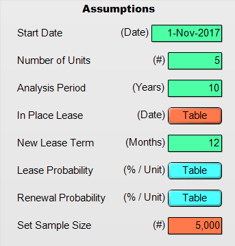
The first three variables are self-explanatory.  The timing of the model is on a monthly basis, so the model constructs the Month index from the Start_Date and the Analysis_Period variables.  See the module, Indexes to find the Month index object.  The In_Place_Lease variable inputs the first and last month for each of the leases in place at the start of the analysis period.  I have selected arbitrary start and end dates, with some very long initial leases, and two of the units are vacant.  Click the button “Table” to view and to change these dates:

The New_Lease_Term is a decision variable for the property owner to decide the lease term for each new lease after the initial leases terminate.  This variable could vary depending upon the unit number or unit type, but to keep things simple it is set to 12 months.  If you would like to change this variable to depend upon the unit number, select the input field and type Table(Unit_Number). Then select the table button that appears.  One of the great advantages of Analytica is its flexibility in adding or removing arrays without interfering with the operation of the rest of the model.

The next two input variables are the lease and the renewal probabilities.  These variables may vary for each specific unit.  The Lease Probability is:

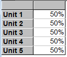
The Renewal Probability looks the same and is also set to a 50% probability of renewal per month and for each unit.  Again, feel free to change these probabilities when exploring the model.

With the above basic assumptions set, the main influence diagram (ID) is pictured below.

Analytica’s influence diagram paradigm allows a visual representation of the model.  The type of each variable is represented by a specific shape, e.g. rectangles are decisions and ovals are uncertainties.  Additionally, the dependencies between variables are indicated by arrows.  See the link above for a further description of an influence diagram.  (If you want to get down and dirty into Influence Diagrams see Howard and Matheson’s classic paper.)  To assist in understanding the ID, I have enabled help balloons.  Just hover your cursor over a node and a balloon will appear with a description of that variable.  For example:

The node In_Place_Lease_Month calculates the month number that each of the initial leases are in at the start date.  In_Place_Lease_End_Month calculates the index value of the Month index that is the last month of the initial leases.  This may seem a little confusing, but what these variables are doing should become more clear below in the code section.  Essentially they help to target the specific month when the initial leases end.  Both of these variables are intermediate variables that are used to calculate the primary variable of interest, the Lease_Month.

The Lease_Month variable is where the simulation for the different possible future occupancy paths occurs.  Below the results for this variable are set to sample view, so that we can see the different leases and vacancies for each run (aka future) of the simulation and for each unit.  (Your results may have different numbers due to the nature of computer simulation.)

In the table above, different possible futures for Unit 4 are shown.  Each cell contains the month number for each lease over time.  So a 0 means that the unit is vacant, and a 5 is the fifth month of the lease.  Note that the first month, 1-Nov-2017, has the number 28 in every cell.  This means that Unit 4 is in the 28th month of it’s initial lease during the first month of the holding period.  The 28 is calculated by the In_Place_Lease_Month variable.

The last month for the initial lease begins at 1-Jan-2018, the 30th month of that lease.  The following month is where the simulation begins for this unit.  On 1-Feb-2018 the model draws a Bernoulli random variable, either 0 or 1, to determine if the lease is renewed, i.e. when the draw results in a 1.  The probability of a 1 is determined by the Renewal Probability.  If the lease is not renewed, the unit becomes vacant for at least one month.  (This can be easily changed, so then the model would draw an additional random variable to determine if another renter signs the lease prior to assigning the unit to vacancy.)

Looking at the above table we see that there are drastically different results for the same unit after the initial lease ends, despite the renewal probability being the same in each simulation trial.  For instance in Run 4, there is only one vacant month after the initial lease ends.  In Run 2, there are no vacant months.  But during Run 7, there are six vacant months, and during Run 6 there are five vacant months.  This is the dispersion problem described above made manifest in a way that traditional lease analysis can never capture.

This same process for determining a renewal or vacancy also occurs after a new lease reaches month number 12.  For example, in Run 2 starting at date 1-Feb-2020 there are six consecutive vacant months, despite the unit being occupied right after the initial lease and two subsequent leases.

One of the great properties of Analytica is that the above simulation is repeated independently for each unit with no additional coding needed.  To view the results for the other units click on the slicer arrow above the table.  Also be sure to alter the total number of units on the property via the assumptions panel. A maximum number of 32,000 units is allowed in this version of the software.

Lastly, let’s look at the Max_Vacant variable.  This node calculates the maximum number of months vacant for each unit and over every run of the simulation.  We see that despite having only a 50 percent chance of a vacancy when a lease ends, it is possible to have long stretches of unoccupied units.  The results are:

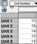
Every unit had a maximum vacancy of more than a year.  While preparing for these downside possibilities is important, first a decision maker has to know they exist.  This downside risk is something which a blended rate analysis will always fail to provide.

Some Code

In this section we will walk through some code to get a feel for how the model works under the hood of the influence diagram.  We will focus on Lease_Month since it is both the primary variable of interest, and has the most complex definition.

The Definition of Lease_Month is the following expression:

Dynamic[Month](

/* First Month */
In_Place_Lease_Month
+ ( In_Place_Lease_Month = 0 ) * Bernoulli(Lease_Probability) ,

/* Other Months */
If @Month <= In_Place_Lease_End_M
Then In_Place_Lease_Month + @Month - 1
Else if ( @Month - 1 ) = In_Place_Lease_End_M
   or Self[Month - 1] = New_Lease_Term
Then Bernoulli(Renewal_Probability)
Else if Self[Month - 1] = 0
Then Bernoulli(Lease_Probability)
Else Self[Month - 1] + 1
)

Line 1, Dynamic[Month] initializes the Dynamic environment in Analytica, and sets the index over which Dynamic will step to be the Month index.  Line 4 and 5:

In_Place_Lease_Month  + ( In_Place_Lease_Month = 0 ) * Bernoulli(Lease_Probability)

is what happens during the first month. The In_Place_Lease_Month calculates the month number that the original leases will be in at the start date of the analysis.   Since any vacant unit will have an In_Place_Lease_Month value of zero there is a draw from a Bernoulli distribution to determine whether the unit becomes occupied or not. This Bernoulli draw is then multiplied by ( In_Place_Lease_Month = 0 ) which is a logical test whether the unit is vacant, 0, or not.  So, as an example, if Bernoulli(Lease_Probability) draws a 1, but ( In_Place_Lease_Month = 0 ) is false, meaning the unit is occupied, then we have 0 * 1 which equals 0, and the draw is not applied for that month.

Note that because In_Place_Lease_Month and Bernoulli(Lease_Probability) both have values that are indexed by the Unit_Number index, the result of the expression on line 4 will also be indexed by Unit_Number.  The programmer does not have to worry about the expression evaluating for each unit on the property, as Analytica does this automatically.  This is an example of the array programming paradigm which greatly simplifies model building.

The next line of interest is line 8 that evaluates the conditional statement:

If @Month <= In_Place_Lease_End_M

The @ symbol in front of Month is the position operator that returns the position (a number) for that month in the index.  So the start date of 1-Nov-2017 has a position equal to 1, and so forth for the other Month elements. This conditional statement determines whether the initial leases have expired or not. If they have not ended, then the lease month is increased by one month via the expression In_Place_Lease_Month + @Month - 1. Note that we deduct 1 since the first month’s position is 1.

If the initial leases have terminated, then the model has to determine when a renewal can occur.  This is the task of line 10, which checks for the final lease month of an occupied unit in the previous month:

Else if (@Month - 1) = In_Place_Lease_End_M
or Self[Month - 1] = New_Lease_Term)

In English this condition evaluates to “If the prior month is equal to the end of the initial leases, or the prior month equals the last month of a new lease”.  If the condition is true, then the next line determines whether the lease is renewed by a draw from the Bernoulli distribution, 0 or 1, evaluated at the renewal probability:

Bernoulli(Renewal_Probability).

If the condition starting at line 10 is false, then we have our final conditional statement:

Else if Self[Month - 1] = 0

which asks whether the unit was vacant during the prior month.  If yes, then it determines whether it is leased or not at the market lease probability via:

Bernoulli(Lease_Probability)

Lastly, if line 13 is false, that is the unit was not vacant in the prior month, then the lease month number is increased by a single month, Self[Month - 1] + 1.

Final Word

This post demonstrated how to simulate the physical occupancy for a multifamily building over time. In the next post, we will use what we have created here to develop a model of rental cash flows subject to unit vacancies. As always, if you have any questions please feel free to email me.