(Note: This post uses Analytica by Lumina Decision Systems.  The free version is here.  Also here is a nice and easy introduction to the language.  You can download the model presented here at 2017-5-25 Lease Up Model )

Introduction

This post will present one method for handling the absorption phase risk for a real estate development.  The absorption phase is the period of time during a development project when the units are actually leased and occupied.  This phase can be critical in making or breaking a project for a variety of reasons.  One important risk during this phase relates to the term of the construction loan and the occupancy requirement needed for the permanent lender to step in and “take out” the construction loan.  If stabilization is not reached, then the lender does not have an obligation to step in and payoff the construction loan.  For example the California Housing Finance Agency requires a 90 percent stabilized occupancy rate for 90 days as a requirement for permanent lending. Thus there can be substantial risk to a developer if the stabilized occupancy is not met prior to the end of the construction loan’s term.  Therefore it is important to understand how different rates of absorption can impact the project.

If they bother to model the lease-up phase at all, many Excel modelers assume constant absorption rates. More determined Excel modelers will use an S-Curve.  This post demonstrates a different approach.  Instead of a deterministic absorption process, such as a constant absorption rate, we will model our uncertainty using Monte Carlo simulation in the Analytica modeling environment.  (Free version of Analytica here.  If you would like to play around with the module presented in this post, see the attached zip.)

Property level absorption analysis is the perfect situation for using simulation because of the uncertainty over when the actual leasing of each unit occurs. Stochastic sensitivity analysis, i.e. using different mean absorption rates in this case, then makes it easier to understand how the absorption rate impacts the project’s feasibility and return characteristics.

While there are many different ways to simulate the lease-up phase, in this post we will use a Poisson process to model absorption by unit type.  A Poisson process counts the number of occurrences of an event in a given time interval.  In this module, we are interested in counting the number of units leased in each month for each unit type.  This approach will work best when there are many units in the development. In our example there are 30 studio units, 40 one bedroom units, and 30 two bedroom units for a total of 100 units.  Since this example is relatively simple, we won’t adjust for seasonality, which can be a factor in an absorption analysis.

Let’s jump to the Influence Diagram to take a look at the model logic:

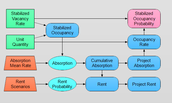
If you download the module I have added help balloons for most of the variables that describe their function.  So just hover your cursor over a node and its unit and description attributes will appear.  To keep this post somewhat concise I am only going to focus on the variables Absorption and Stabilized Occupancy Probability.

Unit Absorption

The Absorption variable simulates the lease-up process over time. As we can see from the diagram, Absorption is dependent upon the following two variables:

1. Stabilized Occupancy – This variable is the number of units for each unit type that we expect to be occupied at stabilization.
2. Absorption Mean Rate – This variable is the rate for the Poisson process. Mathematically it is the expected number of units leased in each month.  Although it is assumed to be a constant variable in this model, in practice it is best to derive this value in one of two ways.  The first, and potentially more accurate but also more complicated approach, is via Poisson regression.  The second method is to elicit a range of values from people with knowledge of the local submarket. I hope to get more in depth on both methods in future posts, as these different approaches to handling model assumptions can be used in many areas of real estate investment modeling.

The definition of Absorption is the following:

Dynamic(
     Min([Poisson(Absorption_Mean_Rate, Over: Unit_Type), Stabilized_Occupancy]),
       INDEX Past_Months := 1 .. @Time -1 ;
       VAR Remaining_Units := Stabilized_Occupancy - Sum(Self[@Time = @Past_Months], Past_Months);
     Min([Poisson(Absorption_Mean_Rate, over:Unit_Type), Remaining_Units])
)

Let’s break down the above definition line by line to understand what is going on.

The first line Dynamic simply initiates the Dynamic function in Analytica. Dynamic is used to model quantities that change over time and that are dependent on earlier time periods. For example, in this model, a unit leased in the previous month is not available to be leased today. Dynamic captures this type of dependency.

The next line is for the first month in the Dynamic array.

Min([Poisson(Absorption_Mean_Rate, Over: Unit_Type), Stabilized_Occupancy]),

The Min([ ]) function with brackets takes the pairwise minimum for the arguments entered on both sides of the comma.  So in this case it takes the minimum of the first month’s Poisson draw, and the Stabilized Occupancy.  The reason for including the pairwise minimum is that we don’t want the Poisson process to draw more than the stabilized level of occupancy.  The function Poisson(Absorption_Mean_Rate, Over: Unit_Type) has two arguments. The first argument Absorption_Mean_Rate tells Analytica to use the value from the variable Absorption Mean Rate as the rate of the Poisson process. Again the rate is thought of as the expected number of units leased in a single month.  Since Analytica is an Array Programming language, we define Absorption Mean Rate := 1..5 which is simply a sequence of integers from 1 to 5 using the “dot-dot” operator.  This allows us to perform stochastic sensitive analysis on the simulation, meaning that Analytica will repeat the simulation for each rate.

The next argument of Poisson is the Over:Unit_Type. The keyword Over tells Analytica to repeat the Poisson function over each value of the index Unit Type. In this case Unit Type is defined as Studio, One Bedroom, and Two Bedroom.  Note that in a more realistic model each unit type may also have their own mean absorption rates. This is not done here, but is easy to add to the model.

The next line of Absorption is:

INDEX Past_Months := 1 .. @Time - 1;

This creates a local index in Analytica named Past_Months.  The goal here is that we want to determine the number of available units after deducting for the units leased in the prior months.  The local index allows us to access all the prior values in the same array (Absorption) up through the last month, which has been already calculated. The local index does precisely this with 1 giving us the first period of the array and @Time - 1 giving the period of the array prior to the current period being calculated.  Again the dot-dot operator is used to construct a sequence of integers between the beginning and ending values.

This local index then works its magic with the next line of code:

VAR Remaining_Units := Stabilized_Occupancy - Sum(Self[@Time = @Past_Months], Past_Months);

This line creates a local variable that uses the local index Past_Months.  Setting @Time = @Past_Months is an example of re-indexing, which gives Analytica tremendous power in handling indexes.  Re-indexing allows the Time index to be replaced by the Past_Months index. The function Sum then sums along the Past_Months index, arriving at the the total number of units leased prior to the present month.

The last line is a near repetition of the calculation for the first Month above. However, the slight difference is that the minimum being taken is over the smaller value of the number of remaining units versus the outcome of the Poisson draw.  This way the model doesn’t absorb more units than are actually available.

Now lets take a look at the output of Absorption in sample view:

This is a four dimensional array (good luck with that in Excel!) indexed by Time(in months), the Absorption Mean Rate (from 1 to 5), the Unit Type, and a new index called Run.  I have set the sample size to 5,000, which means that the simulation will perform 5,000 different trials.  Run is an index of numbers from 1 to 5,000.  For each value of Run, Analytica performs a Poisson draw representing the number of units leased in each month.  For example in Month 2 during the second simulation run, 5 two bedroom units were leased. As noted above, Analytica will perform this calculation automatically for each value of Absorption Mean Rate and Unit Type.  (This process is called array abstraction.)  Considering all four dimensions, this array has 1.8 million cells.  In Excel one would need to use VBA for an object of this size. Analytica makes it almost effortless.

Stabilized Occupancy Probability

Now one of the goals of this module is to determine how different absorption rates affect a project’s ability to meet the permanent lender’s stabilization rate by the end of the construction loan term.  This question is answered by the Stabilized Occupancy Probability variable, or SOP for short.  SOP has two parent nodes, the Stabilized Vacancy Rate and the Occupancy Rate.  The Stabilized Vacancy Rate is the vacancy rate at stabilization, and the Occupancy Rate is the percent of the project occupied during each month.

The definition of SOP is:

var stabilized_occupancy_rate := 1 - Stabilized_Vac_Rate;
Probability(Occupancy_Rate >= stabilized_occupancy_rate )

Again a local variable is used, this time for the stabilized occupancy rate. (In a larger model I would have this in a separate global variable.)  The next line uses Analytica’s Probability function.  This function evaluates the probability for the test condition to be true for the Monte Carlo sample drawn.  In this case the test condition is Occupancy_Rate >= stabilized_occupancy_rate, so in English we are looking at the probability that the occupancy rate will be greater than or equal to the stabilized occupancy rate over time.

The result is:

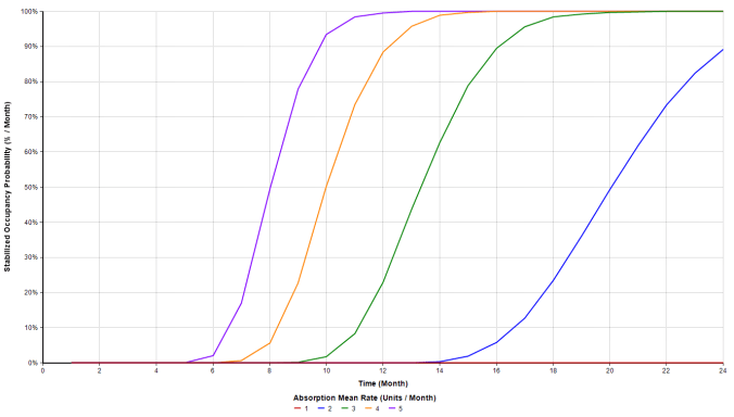
This variable tells us the probability of meeting our stabilized occupancy requirement for each month.  If an average of one unit is leased per month then the probability of meeting the stabilization requirement is zero for every month.  Clearly if more units are leased per month, the probability of meeting the stabilized occupancy level increases and happens sooner.  From this graph it’s easy to see that with a mean rate of 3 or more units leased per month the stabilization rate will be met before the construction loan comes due at month 24.  This graph is a nice and easy representation of our absorption risk.

Conclusion

This post presents a simple model for handling uncertainty over the absorption phase in a real estate development project.  The centerpiece of this approach is the simulation of the project’s absorption, instead of assuming a deterministic absorption pattern as is typically done in real estate modeling.

In the next post, I highlight reasons for why modelers should prefer Monte Carlo simulation to the traditional, deterministic, approach to real estate modeling and demonstrate a Monte Carlo model that simulates a property’s vacancy process over time.

As allows, if you have any questions feel free to email me.