Introduction

This post provides an example of how to value a natural gas swing option using the Least Squares Monte Carlo method (LSM). Swing options are common option contracts in the energy industry. They allow managers flexibility in determining both the timing and quantity of delivery for energy and related commodities. These option contracts are important because of the high level of uncertainty in the volume needed to meet supply and demand as these conditions change rapidly over time. The options are called “swing” options because when the option is exercised the quantity can vary, i.e. be “swung”, between a high and a low volume level.

As an example of why swing options are useful consider a power utility in Los Angeles that must prepare for the summer months. During the summer there is the risk of a heat wave hitting the city on any given day. A heat wave will cause a spike in electricity usage and energy prices as people crank up their air conditioners to stay cool. A swing option in this situation would give the power company the ability to hedge their fuel needs on these hot days without having to pay the high daily spot price. (European and American options could be used but they would be excessively expensive due to their exercise features. See Jaillet et al (2004) for a discussion of the relationship between the three option types.)

The valuation method used in this post is LSM. LSM is a powerful technique that combines Monte Carlo simulation with regression analysis and dynamic programming. For further discussion and examples on LSM see my earlier posts where the LSM method is used to value a mine and also value a pharmaceutical patent. Additionally see this nice answer on the StackExchange Quant Finance discussion describing the LSM algorithm in plain English. Lastly Glasserman (2004) chapter 8 has an in depth discussion of how to solve options with early exercise features using the LSM approach along with several other Monte Carlo techniques and how they all fit together.

The model here was created in Analytica, which remains my favorite modeling language. You will need the free version to open and change the model. You can download the swing options example here:

A comparable model in Matlab, on which my example is based, is demonstrated at the MathWorks website here.

The Matlab model is a little more extensive than my example, as it also demonstrates using a smoothing spline regression as an alternative to approximating the continuation value with a power series regression. Additionally the Matlab example demonstrates how to bound the value of the option between upper and lower bounds using European and American option values. I might add these features in a separate post, so stay tuned. The price process is the same in the Analytica model and in the Matlab example. However unlike the Matlab example, the model here allows the user to enter the order of the approximating power series, which can only be of order three in the Matlab model.

While Analytica is my favorite modeling environment, a plan for the summer is to redo many of my posts in Julia, which is a great open source alternative to Matlab. (An example Julia model using the LSM approach for option valuation is here. However that model is not a swing option, just a standard American option. For benchmarks comparing Julia to Matlab see here.)

The Model

As mentioned above the example here is a natural gas swing option which assumes a daily contract quantity and a given number of exercise rights during the contract term when the quantity can be “swung” above or below the daily contract quantity. The model assumes 5 exercise rights, as in the Matlab model, but the user can change this assumption. The contract term is one year and the option can be exercised on any day during the year. The option can be exercised only once per day even if multiple exercise rights remain.

Below is the user panel for this model, I won’t go through each of the inputs as help balloons are enabled so just hover your cursor over an input’s name and a description will appear. Additionally the inputs generally mirror the inputs of the Matlab model so refer to that post for specific details. Note that the user is free to change any of these assumptions.

The payoff from exercising the swing is determined by the price of natural gas. The (risk neutral) natural gas price evolves over time according to a mean reverting one factor Hull-White stochastic differential equation. See the Matlab post for the actual equations. Below are 500 possible prices over the one year simulation period:

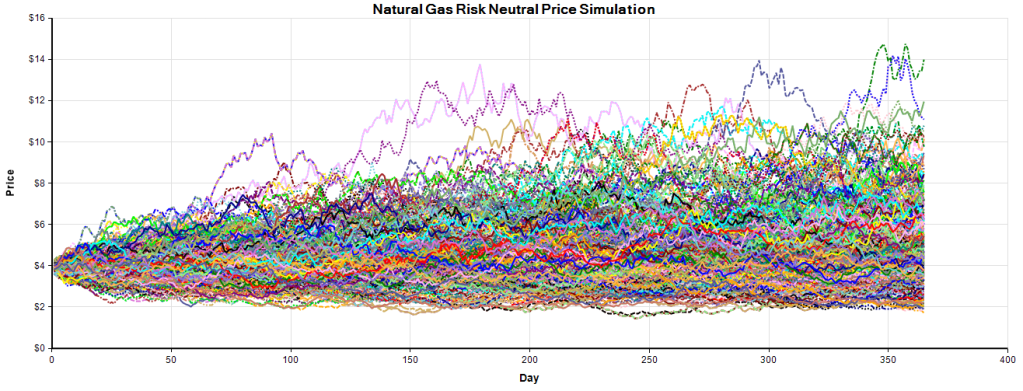
This chart is very similar to the Matlab output as we should expect. Despite the mean reversion inherent in the process there is substantial uncertainty about future prices just as we observe in actual price data. Note that one advantage of the LSM is that it is not wedded to any particular stochastic process used to simulate the underlying asset prices. So this mean reverting process could be swapped out for another process without affecting the LSM algorithm, if another process better fits the data.

Solution Method

The LSM solution procedure for this type of option uses a dynamic programming approach to compare the trade off between not exercising today and receiving the continuation value versus the payoff from exercising today plus the continuation value of having one less exercise right tomorrow. (Note that when the number of exercise rights is zero, the continuation value is also zero.)

Seeing the algorithm may help make sense of it, so it is below. I added comments in green to try and explain each variable (denoted by the “local” key word). Additionally the procedure starts in the last period, the Terminal State Value, and works backwards as denoted by the Self[Day+1] keyword which is the value of the option one day in the future.

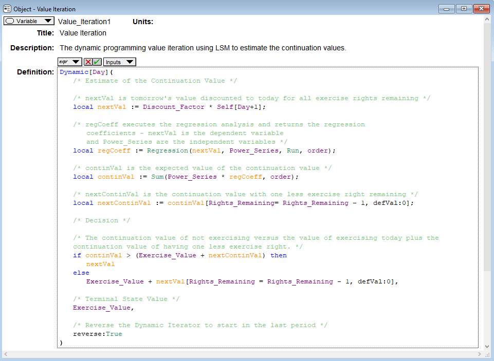
Analytica’s Dynamic function acts like a “for” loop and iterates over each day starting from the maturity date (the reverse keyword is true). Note that in the decision section of the algorithm continVal and nextContinVal, the estimated continuation values from the regression analysis, are used to make the decision but nextVal is used for the actual valuation. The reason for this is technical and beyond the scope of this blog post, but it is a means to control for biases in approximating the true value at each stage. See Glasserman (2004) chapter 8 referenced above for more on high and low biases.

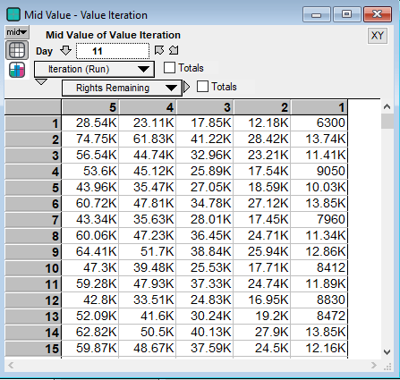
The result of the above code is a three dimensional object containing the option values for each day, simulation run and the number of options remaining. As an example, the Day 11 option values are below:

There is one last step to the algorithm as the code above estimates the option value for each day during the year but not at the settlement date. The final step of the LSM algorithm is below and it simply takes the average across all simulation runs on the first day with five exercise rights remaining (the number of rights in existence at the settlement date).

Results

For a 3rd order polynomial regression the Matlab model gives an estimate of $56,943 compared with the Analytica model’s estimate of $57,297. Additionally I allow the user to enter the order of the approximating polynomial, so for a 5th order polynomial the estimated option’s value is $59,179, which is very close to the Matlab model’s cubic spline regression estimate of $60,757. Thus these models are in agreement as we expect.

Well that is one approach to valuing a swing option. If you have any questions or comments feel free to email me.