To become significantly more reliable, code must become more transparent. In particular, nested conditions and loops must be viewed with great suspicion. Complicated control flows confuse programmers. Messy code often hides bugs.

— Bjarne Stroustrup

https://www.stroustrup.com/Software-for-infrastructure.pdf

In the previous post I discussed the valuation of energy swing options, which I created in the Analytica modeling language. However I didn’t reproduce any of the Matlab code to compare it to the Analytica code that I did include. So below is a portion of the Matlab code needed to value the swing option next to the corresponding Analytica code.

I won’t go through the complete code, instead let’s just look at the code needed to compute the backward induction portion of the LSM algorithm. I think the general point of how much clearer Analytica’s syntax is and how much easier Analytica is to work with carries through to the rest of the Matlab code. If you would like to see the complete Matlab function used to compute the swing option’s value, then do the following: on the MathWorks website click the Try This Example button in the upper right corner and then in any gray code box enter:

edit hswingbyls

Press CTRL+ENTER and the code for the entire function should appear.

So let’s turn to the backward induction iteration in each language. Below is the backward induction in Matlab:

%-----------------------------------------
% 2. Longstaff Schwartz backward induction
%-----------------------------------------

% Backward induction
% TimesLS(j) never contains Settle or last exercise date because
% (1) Exercise is not possible at Settle
% (2) Last exercise date was already processed above
for t=nTimes:-1:1

    % Copy values from previous time step
    U_prev = U;
    U = nan(NumSwings+1,size(S,2));

    % Variable to hold payoffs
    h = nan(size(actions,2),size(S,2));

    % Loop for each possible right. Index is r+1 (includes 0).
    % r is possible rights remaining. i.e. on second exercise day,
    % possibly only one exercise could have been exercised so far.
    for r = max(NumSwings-t+1,0):NumSwings

        if r == 0
            % No exercise left
            U(1,:) = 0;
            continue;
        end

        % Calculate discount factor from date t to t+1
        RS = intenvset(RateSpec,'StartTimes',TimesLS(t),...
            'EndTimes',TimesLS(t+1));
        D = intenvget(RS,'Disc');
        
        % Determine continuation value for one less right
        X = S(t,:)';
        Y = D.*U_prev(r,:)'; % Note r is one less right
        if useSpline
            C_hat = csaps(X,Y,P,X)';
        else
            OLS = [ones(numel(X),1) X  X.^2 X.^3] \ Y;
            C_hat = F(X,OLS(1),OLS(2),OLS(3),OLS(4))';
        end

        % Determine optimal strategy if exercised
        for a = 1:size(actions,2)
            h(a,:) = payoff(actions(a),Strike(t),S(t,:))+C_hat;
        end
        [hmax,I] = nanmax(h);

        % Determine continuation value if not exercised
        Y = D.*U_prev(r+1,:)';
        if useSpline
            C_hat = csaps(X,Y,P,X)';
        else
            OLS = [ones(numel(X),1) X  X.^2 X.^3] \ Y;
            C_hat = F(X,OLS(1),OLS(2),OLS(3),OLS(4))';
        end
        if t == nTimes && r == NumSwings && LSplot
            plot_cont(X,Y,C_hat,useSpline);
        end
        
        % Determine value given optimal exercise policy
        exercise = hmax > C_hat;
        U(r+1,~exercise) = Y(~exercise);
        U(r+1,exercise) = ...
            payoff(actions(I(exercise)),Strike(t),S(t,exercise))+ ...
            D.*U_prev(r,exercise);
    end

end

The above code computes the swing option values for each number of option rights remaining, in each time period, and along each simulation run using ordinary least squares to approximate the continuation values of the option. Now let’s look at the Analytica code that does the same thing (if the code below is hard to read click here for an enlarged image):

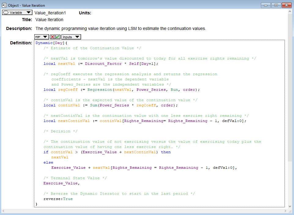
Even though there are a few extra lines in the Matlab code doing additional work (such as “if usespline”), I think this is a very fair comparison that demonstrates how much easier it is to code models in Analytica.

As the Stroustrup quotation that begins this post emphasizes, a key to code reliability is transparency. The Analytica code is much more transparent than the Matlab code. Two key differences between the languages in this example are the lack of for loops in Analytica and Analytica’s use of explicitly named indexes. While Matlab is an array programming language, Analytica is even more so. Instead of having three iterators (i.e. for loops) as in the Matlab model, the only iterator we need for this model in Analytica is Dynamic, which simply starts in the last day and then steps backwards day by day. Analytica’s array abstraction and index operations do the heavy lifting to handle the calculations along the simulation index and the swing rights remaining index. Thus in many cases Analytica avoids nested conditionals and for loops, which eases the cognitive burden on the programmer and modeler. (Note that Analytica does have for loops if you really need them, but they are typically not used because of these other features of Analytica.)

Also since Analytica’s indexes are explicitly named, e.g. Rights_Remaining, we don’t worry about the shape of the objects as we do when using Matlab, which again greatly increases code transparency and reliability in Analytica. To see this notice that the Matlab code includes several apostrophes, ‘, denoting a transposition and reshaping of the object. All of these transposes slows down our reasoning about the model’s logic as we have to re-orientate the object in our heads (at least I do) and this process increases the potential for bugs to creep into the code. Instead, in Analytica, we just think about how to match values along an index. This is much more natural. I highly recommend the Analytica tutorial on Arrays and Indexes, which provides a good example of how indexes work in Analytica and their power.

Another advantage of Analytica over Matlab that I did not touch on in the previous post that also reinforces the principle of code reliability through code transparency is the diagrammatic model building. In Analytica models are represented as a series of nodes and arrows connecting the nodes. This is called an influence diagram. The shapes have meaning as well, where the orange trapezoids here represent inputs and assumptions, the blue rounded rectangles are intermediate calculation nodes and the reddish hexagon is the objective that we want to calculate. Arrows connect dependencies and inputs for calculations, e.g. Exercise Value is a function of the Swing Up, Swing Down, and Price Spread values. Below is the main part of the swing option model that includes the backward induction iteration discussed above (which is the Value Iteration node):

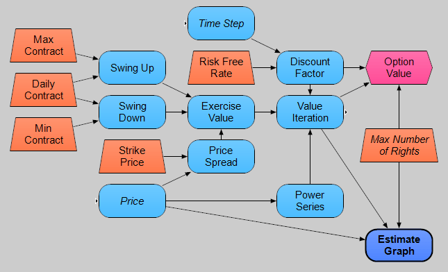
This diagram helps our understanding of the model during both model creation and many months later when we want to reuse a model. With the influence diagram we have an immediate conceptual map of the model and this helps us both remember, and if necessary relearn, the model quickly. I cannot express how useful this is as sometimes it is months before I have to reuse a model. While modeling with nodes and diagrams did feel unusual at first, it has quickly taken over how I think about modeling in general (and yes I have even had dreams of influence diagrams).

Anyways that’s all for now, feel free to email me with any questions or comments.