Introduction

Recently I gave a talk on real options valuation using the Least Squares Monte Carlo method (LSM). LSM is a variant of Regression Monte Carlo (RMC) methods within the field of approximate dynamic programming (ADP). The goal of ADP is to overcome the “curse of dimensionality” that plagues traditional approaches to solving sequential optimization problems (e.g. Markov decision processes). The curse of dimensionality refers to the exponential increase in storage and computational effort as the size and complexity of the problem increases.

The application that I discussed in the real options talk was a real estate development where the project manager had the option to switch between building the project, suspending construction, or even abandoning the project if market prices or construction costs turned sufficiently unfavorable. However these RMC methods have much wider applicability. Thus, this post demonstrates a similar technique applied to a stochastic storage problem, specifically the valuation and control of a natural gas storage facility.

In general stochastic storage problems focus on the optimal use of an inventory that is both limited in capacity and subject to price or demand uncertainty. An excellent paper discussing stochastic storage problems is Ludkovski & Maheshwari (2020) (henceforth “L&M”). (Note all references are at the end of this post with links to a PDF copy.) The authors devise a general statistical learning framework to solve these problems. The paper applies the framework to solve three natural gas storage problems and an electricity micro-grid storage problem. The model I present below is calibrated to their first natural gas storage example, since this is a good introduction to the field.

As far as I know the original approach to natural gas storage valuation was pioneered by Boogert & de Jong (2008). Their grid discretization method with piecewise polynomial regression is still the primary method used to solve these models and it is what I use below. For alternative approaches including non-parametric methods see L&M referred to above.

To download the example model click the button below. You will need the free version of Analytica 101 to view and modify the model.

My post with general background information on real options and dynamic programming is here. For other examples on this blog of approximate dynamic programming and real options analysis a list of posts is here.

For the remainder of this post I will focus on discussing the model, its influence diagram and some graphs. Influence diagrams are an efficient way to show dependencies between variables. To see the definitions of each variable just double click a node in the model.

The Model

The setting is a natural gas storage facility, in this case a salt cavern. The operator can inject or withdraw gas, as well as do nothing, in each time period. Inventory is thus a state variable that factors into the valuation and optimal control of the storage facility. Since the operator influences the inventory level through its actions this state variable is called an endogenous state variable. The inventory in this model is a discretized grid of points. L&M discuss alternatives to discretization for higher dimensional problems.

The rates of gas injection and withdrawal are subject to the hydrodynamical properties of the cavern and depend on the current level of inventory. For more on the hydrodynamics of gas storage and the derivations of the injection and withdrawal equations see Thompson et al (2009).

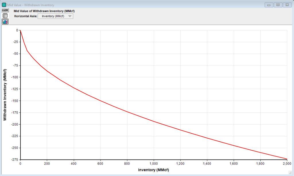
Another assumption for this model is that the maximum quantity of gas will be injected or withdrawn when either action is chosen. This is the so called “bang-bang” solution. Optimization of injected or withdrawn quantities can also be included but tend to have only a minor impact on valuation, see Bäuerle & Riess (2016) as well as Thompson et al. (2009). Below is a graph of the quantity of withdrawn gas at each inventory level. Clearly it is a nonlinear function of inventory level.

In addition to the inventory, the control and valuation of the facility also depends upon a mean reverting gas price process. The price is considered exogenous because the operator does not influence gas prices directly. Bäuerle & Riess (2016) extend this simple mean reverting process to a more realistic regime switching process. One of the great features of RMC models is that the same solution algorithm for valuation and optimal control applies independently of the chosen exogenous price process. So it is easy to test different exogenous processes. Below is a chart of the simulated gas prices for the three year period.

As can be seen in the chart above despite the price process being mean reverting there is a high degree of variability in the price over time.

Turning to the rest of the model, below is a visual layout of the important model components. So far I have discussed the inventory process and the price process:

The next part of the model to discuss is the valuation analysis. There are four modules on the diagram above that perform the valuation analysis. The first module, Terminal Valuation, computes the value of the facility in the final time period. In this example there is a penalty for the facility having less than a contractual terminal amount. The penalty looks like a hockey stick:

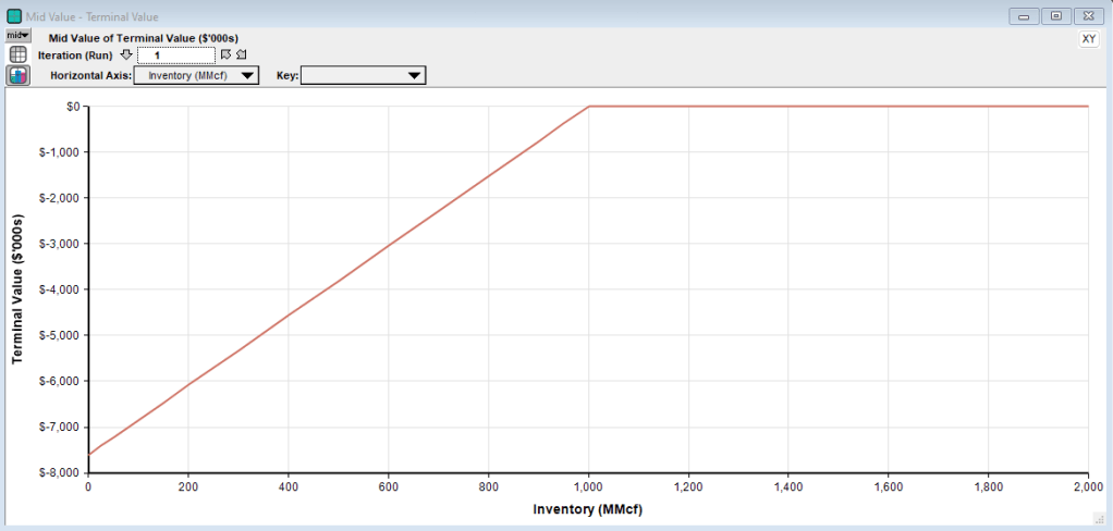
The terminal value serves as an initial value estimate (boundary condition) from which we can begin the dynamic programming algorithm.

The next module for the valuation is Regress Basis, which calculates the regression basis used to estimate the continuation value during backward induction (dynamic programming). For this example the basis is simply a third order polynomial regression for each inventory grid level. The next module, Dynamic Program, is where the fun really occurs. This is the core part of the RMC algorithm. The diagram is below.

The influence diagram allows us to conceptually walk through the valuation process. The variable Value Iteration holds the per period estimate of the facility’s value. It is initially set to the terminal value. The value of Value Iteration is then discounted in Discount Value and the OLS coefficients are estimated from the current basis (the third order polynomial of prices in that period) in OLS Coefficients. The continuation value, Continue Value, is just the inner product of the current basis and the estimated OLS coefficients. A continuation value is calculated at each inventory grid point as there are different coefficients for each grid point.

Next, since we are using a grid for the inventory, an interpolation is performed to calculate the value of the inventory after an injection or withdrawal action as these points will be off of the grid. (See Bäuerle & Riess (2016) for a method to include the injection and withdrawal inventory points in the grid.) The current reward, which is the cash flow from injecting and withdrawing, is then added to the interpolated continuation value to form the Bellman equation in the eponymously named node, Bellman. Value Iteration then maximizes the Bellman equation with respect to the best action, i.e. inject, do nothing, or withdraw, and that is the new estimate of the facility’s value. This process is repeated from the final time period until the first time period.

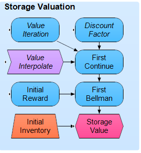
The final module of the valuation analysis, Valuation, forms one last Bellman equation for the initial period and then maximizes over the actions. Here is this module’s influence diagram. The variable First Continue is the continuation value for transitioning from time period 0 to period 1. It is calculated by averaging the Value Iteration variable across all simulation runs, discounting, and interpolating.

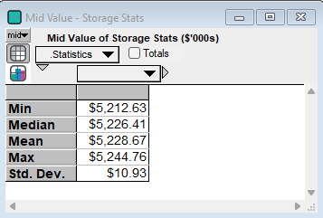
Below are the statistics of running the model ten times with different seeds. They are inline with the results of the L&M paper.

Operating Policy

In many situations we are interested in valuation and also the sequence of optimal actions in managing a project. So in this case at each time period, given the inventory level and the price, the question becomes what action should be taken. This is called optimal control. RMC algorithms provide us with the ability to estimate optimal controls. On the Dynamic Program module diagram above there is a coefficient called Coefficient Sequence. This variable holds the estimated OLS coefficients at each time point and for each inventory level. Using these coefficients we can then estimate the per period continuation value to derive a control. See the influence diagram below:

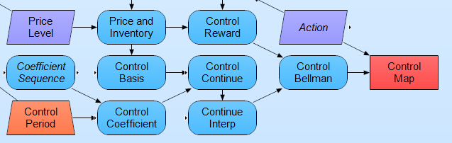
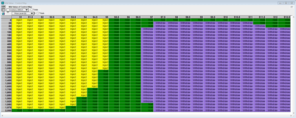
The control map is determined from optimizing the control Bellman equation for the particular time period. This can then give us a table of optimal actions for each price-inventory state pair as we see below:

Note on the TvR Algorithm

In previous example models I used the LSM regression Monte Carlo method. Since I wanted to replicated the L&M paper for this model, I have employed the same TvR regression Monte Carlo method that the paper uses. TvR is an abbreviation for the original authors Tsitsiklis & van Roy (2001) and their approach to solving these optimal stopping/switching problems. The LSM and TvR algorithms are related as they are both look-ahead strategies that use future cash flows in the estimation of the value function. The difference is that TvR looks ahead only one period while LSM looks ahead all the way to the terminal period. Thus LSM uses more information from the future simulated cash flows in estimating the pathwise values. I have built this natural gas storage model using the LSM method and it leads to about a 2 percent increase in value. For an extensive analysis of both LSM and TvR see Egloff (2005). TvR actually provides a lower bound on the estimated value. There are methods to calculated upper bounds, called duals, which I shall present in a future post. In practice LSM is usually preferred.

Conclusion

And that is the basic model of valuing a natural gas storage facility. If you have any questions or comments feel free to email me.

References

Bäuerle, N., Riess, V. Gas storage valuation with regime switching. Energy Syst 7, 499–528 (2016). (PDF)

Boogert, A., Cyriel de Jong. Gas Storage Valuation Using a Monte Carlo Method. The Journal of Derivatives Feb 2008, 15 (3) 81-98. (PDF)

Egloff, D. “Monte Carlo algorithms for optimal stopping and statistical learning.” Ann. Appl. Probab. 15 (2) 1396 – 1432, May 2005. (PDF)

Ludkovski, M., Maheshwari, A. Simulation methods for stochastic storage problems: a statistical learning perspective. Energy Syst 11, 377–415 (2020). (PDF)

Thompson, M., Davison, M. and Rasmussen, H. (2009), Natural gas storage valuation and optimization: A real options application. Naval Research Logistics, 56: 226-238. (PDF)

J. N. Tsitsiklis and B. Van Roy, “Regression methods for pricing complex American-style options,” in IEEE Transactions on Neural Networks, vol. 12, no. 4, pp. 694-703, July 2001, doi: 10.1109/72.935083. (PDF)