In the previous post I demonstrated how to web scrape data from a website with the intention of using the data as part of a geographic information system (GIS) data analysis pipeline. The data that we scraped are the addresses of all CVS pharmacies in the US. Now that we have the data we need to translate these addresses into longitude and latitude coordinates to be useful for GIS analysis. This conversion process, called geocoding, and some basic proximity analysis, i.e. estimating distances, are the subjects of this post. The final layer will be to add demographic and economic data to the census blocks that are used here. But I will save that piece for another post.

PostGIS is my GIS platform of choice and what I will use in this post. PostGIS is a GIS extension to the popular open source relational database management system PostgreSQL (Postgres). PostGIS provides special data types and functions for the manipulation of spatial data. You will see several of these functions in action in this post. What makes PostGIS a great tool for GIS modeling is its complete integration with the rest of the Postgres ecosystem.

PostgreSQL Background

If you have never used Postgres or a SQL database, let alone PostGIS, then the place to start is Practical SQL by Anthony DeBarros. This book is excellent. DeBarros covers everything from installing Postgres to demonstrating several PostGIS examples. For PostGIS resources specifically, I recommend this online introduction and the bible of PostGIS, PostGIS in Action by Obe and Hsu. And of course here is the PostGIS documentation.

Tools

This post uses pgAdmin to execute commands. However if you prefer a CLI over pgAdmin, then I highly recommend you check out pgcli . Pgcli includes code highlighting and code completion making it easier to use than psql.

Since pgAdmin provides basic functionality for generating maps with the geography data type, the primary spatial data type used in this post, I won’t discuss in any detail other mapping tools. That being said QGIS is very good for constructing sophisticated and sharp looking maps. Additionally QGIS connects to Postgres/PostGIS easily.

Since this post will be long enough, I won’t go through creating the database and the schema (cvspharm here), loading (see the \copy command) the scraped CVS addresses, installing PostGIS, and installing the TIGER geocoder (for Linux/WSL users see here).

Geocoding CVS Pharmacy Addresses

Geocoding is the process of translating the textual representation of an address into geometric or geographic coordinates, such as longitude and latitude. These coordinates will form the basis of the proximity analysis, where we estimate distances, below. However before the geocoding process can begin the data and database table must be prepared.

With the US store address data loaded into the database in a table called cvspharm.us_stores, the data preparation steps are to determine the geographic region of interest, create a table to hold geocoded data, and then subset the relevant data from the data table holding the national data. For this post only the stores in Massachusetts are used. The code below creates the table to hold the MA geocoded data:

create table cvspharm.ma_stores (
    addr_id bigserial primary key not null,
    rating integer,
    address text,
    norm_address text,
    pt geometry
);

The column addr_id is a unique identifier for each address. The column rating is the rating that the geocoder returns. It is an integer estimate of how accurate the geocoder is in finding the appropriate coordinates. A rating of zero is a perfect match while higher ratings indicate that the geocoder is having difficulty finding appropriate coordinates for the address. The address column is just the raw text address from the web scraper. The column norm_address will hold a “pretty print” version of the address that the geocoder returns. It can be used to compare the address the geocoder “sees” with the inputted address. And lastly pt holds the coordinates returned by the geocoder as a geometry spatial data type. Spatial data types will be discussed more below.

With the geocoding table in place, the Massachusetts store addresses are loaded into the address column in the table above. Postgres provides several functions and methods to search strings. The like operator is used here to match a substring of each address in the usa_stores table to subset the rows with Massachusetts stores:

insert into cvspharm.ma_stores(address)
select address
from cvspharm.usa_stores
where address like '% MA %';

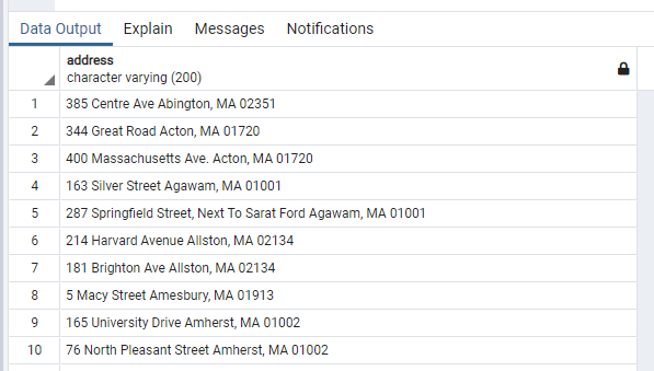
Note again that cvspharm is the schema for the CVS pharmacies. The above code returns 413 store addresses in Massachusetts and places them into the table cvspharm.ma_stores. Below are the first 10 addresses:

With the target data in place, the next step is to geocode each pharmacy’s address.

However we cannot just map the raw addresses from the web scrape into their coordinates. First the addresses need to be normalized into a format that the geocoder understands. This normalization (also called standardization) process decomposes the text of an address into its elements such as street number, street name, and zip code. See the documentation for the normalize_address function for more information. As an example the code

select normalize_address(address)
from cvspharm.ma_stores
limit 10;

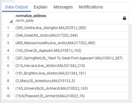
returns a composite data type for each record called a norm_addy with each address’s elements decomposed into appropriate fields. See below:

To make the decomposition of an address into the norm_addy data type’s fields more explicit execute the following code:

with mass_ten as (
	select normalize_address(address) as adrs
	from cvspharm.ma_stores
	limit 10
)

select (adrs).*
from mass_ten;

This returns:

Each column in the above snippet corresponds to a field of the norm_addy composite data type used during geocoding. Not all fields are used with every address.

It is now time to perform the geocoding for each store in Massachusetts. The following code updates the ma_stores table, normalizes the addresses, geocodes the normalized address, and returns the results of the process to the appropriate column. The code is below:

update cvspharm.ma_stores
set
	(rating,norm_address,pt) =
	(coalesce(g.rating, -1), pprint_addy(g.addy), g.geomout)
from cvspharm.ma_stores as a
left join lateral geocode(a.address, 1) as g
on g.rating < 25
where a.addr_id = cvspharm.ma_stores.addr_id;

Much of the code is standard SQL with the geocoding happening on line 6. There the code uses the lateral key word allowing the geocode function to reference the address column of the table aliased by a. The first argument passed to geocode is a.address, which is the raw address text from the web scrape. The geocode function standardizes the addresses automatically. The second argument, the number 1, is the number of results to return for each address. Since only the highest rated geocoding is needed, then 1 is used. The next line finishes the join with on g.rating < 25 which means that only results with a rating better (lower) than 25 are kept.

The results for the first ten addresses is below:

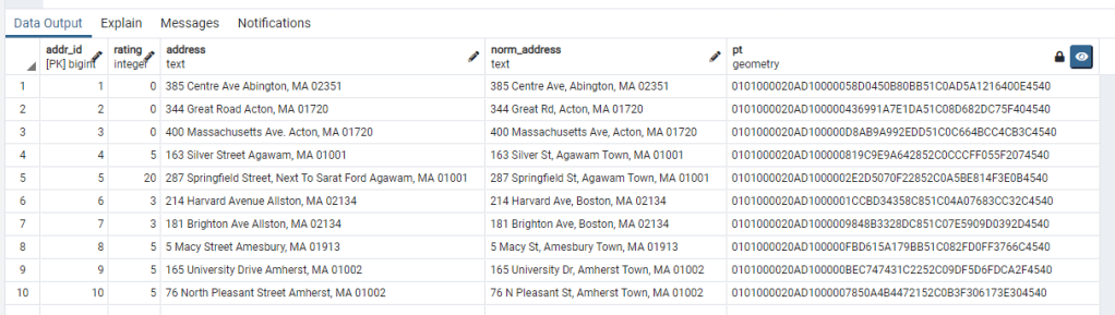
Most of the ratings are low (again this is good) with the one exception being line 5. In this row note the difference between the raw text address that was scraped from the CVS website in column address and the normalized address returned from the geocode function in column norm_address. The raw address contained additional text that was not used by the geocoder.

In column pt each address is now represented by a hexadecimal number representing the geocoded coordinates of the address. For easier reading the hexadecimal numbers can be converted to longitude and latitude with the following code:

select
	norm_address,
	st_x(g.pt) as longitude,
	st_y(g.pt) as latitude
from cvspharm.ma_stores as g
limit 10;

Which looks like the following:

Unfortunately the geocoding was not successful for every text address from the web scrape. In this case 51 addresses had a rating of 25 or above assigned to it from the geocoder. These geocoding misses are assigned a -1 above. The code to count the missed geocodings is below:

select count(*)
from cvspharm.ma_stores
where rating = -1;

When a miss occurs the geocoder does not assign a normalized address nor does it convert the address to a geometry data type as can be seen in the snippet below for 3 of the 51 misses:

In an actual application these misses will have to be handled, but for this blog post they will simply be dropped. So with the geocoding complete, it is time to turn to the actual proximity analysis.

Proximity Analysis

Proximity analysis is a collection of methods for answering distance related questions like nearest neighbor searches. As the linked Wikipedia article discusses, this type of analysis is very important for site location analysis and business intelligence applications. In this section several basic examples of proximity analysis will be demonstrated. But first spatial data types needs to be discussed, as using the wrong spatial data type can send a proximity analysis off the rails quickly.

Spatial data comes in four basic types, geometry (planar like a map), geography (spherical like a globe), raster (multi-band cells like pixels on a monitor), and topological (relational like networks). Geometry and geography data types are the types relevant for the analysis below and the focus here, so the other types are not discussed.

Both geometry and geography data types can be used with different spatial reference systems (SRS). The SRS keeps track of how the different points within the coordinate system relate to each other. Mixing systems or using the wrong system for an analysis will result in nonsense, so it is important to keep the SRSs straight. In PostGIS the SRS is managed through a spatial reference ID number (SRID) that corresponds to the EPSG code. For example to see the SRID returned from the TIGER geocoder used above run the following code, which will return an SRID of 4269:

select st_srid(pt)
from cvspharm.ma_stores
limit 1;

SRID 4269 is the NAD83 coordinate system. The units of SRID 4269 are in degrees. So measuring distances with PostGIS functions like st_distance would return degrees, which is not relevant for a proximity analysis. Therefore the CVS pharmacy geometry data points must be transformed to a different SRS. Here the geography data type with SRID 4326 (the main geography coordinate system) will be used since distances are measured in meters in this system.

The code below transforms the geometry data in the MA pharmacies table into a new table cvspharm.ma_geog holding a geography data column and an ID column. The ID column is used to maintain a correspondence with the text addresses held in the original table. (The addresses could be copied but duplicating data is typically bad practice.) The function st_transform takes a geometry as its first argument and an SRID as its second argument, here 4326. The :: operator then casts the transformed geometry data into geography data. Additionally, on the last line, the addresses that the geocoder missed are dropped as discussed at the end of the last section.

select 
	addr_id,
	st_transform(s.pt, 4326)::geography as geog
into cvspharm.ma_geog
from cvspharm.ma_stores as s
where s.rating >= 0;

The results of the above operation return a column of address ids and the geography data records, below are the first five:

Since the data type is geography with SRID 4326 representing longitude and latitude coordinates, pgAdmin can map the points using OpenStreetMap. Below is a map of the CVS pharmacies in Massachusetts:

From the map we see several patterns, such as clustering in major cities like Boston, Springfield, and Worcester as well as pharmacies near off ramps and road junctions. But to really perform proximity analysis a reference point is needed.

The following code creates just such a reference point, Fenway Park in Boston, MA. The code geocodes the text address, transforms the reference system from SRID 4269 to 4326 and then casts the geometry data type as geography:

select
	rating,
	pprint_addy(addy) as norm_address,
	st_transform(geomout,4326)::geography as geog
into fenway_park
from geocode('4 Jersey St, Boston, MA 02215',1);

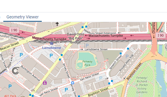
The blue circle at the intersection of Jersey Street and Van Ness Street in the image below is the point representing Fenway Park:

With Fenway as the reference point, the following code uses the st_distance function to find the distance between Fenway and each CVS pharmacy in Massachusetts. Because st_distance returns meters the value is divided by 1,000 and multiplied by 1/1.6 for a short hand conversion to miles. The results are ordered nearest to farthest as can be seen in the image below the code. The inner join is used to return the text address.

select 
	stores.norm_address,
	(st_distance(s.geog,f.geog) / 1000.0 * 1/1.6)::numeric(5,2) as miles_to_fenway
from cvspharm.ma_geog as s
cross join fenway_park as f
inner join cvspharm.ma_stores as stores
on s.addr_id = stores.addr_id
order by miles_to_fenway;

It is important to recognize that the distances returned by st_distance are not driving distances, but the minimum geodesic distance. If driving distances are important then the pgRouting extension can be used. But I will not cover that extension in this post. For many site location analyses PostGIS distance functions are sufficient.

Below are the 10 furthest CVS pharmacies in MA from Fenway park.

select 
	stores.norm_address,
	(st_distance(s.geog,f.geog) / 1000.0 * 1/1.6)::numeric(5,2) as miles_to_fenway
from cvspharm.ma_geog as s
cross join fenway_park as f
inner join cvspharm.ma_stores as stores
on s.addr_id = stores.addr_id
order by miles_to_fenway desc;

In addition to finding store distances from a point, another question to ask is how many stores (and which ones) are within a certain distance from a point. These questions are answered with the st_dwithin function. For example the code below counts the number stores within 5 miles of Fenway:

select
	count(addr_id)
from cvspharm.ma_geog as g
cross join fenway_park as f
where st_dwithin(f.geog, g.geog, 5.0 * 1.6 * 1000);

The answer is 60.

Conclusion

Well that is the basics of geocoding and proximity analysis in PostGIS. Naturally these questions become more interesting with demographic and economic data. But those questions will have to be handle another time. If you have any questions feel free to email me.