Introduction

An essential element and input into a Wind Energy Feasibility Study is an accurate forecast of the wind resource at the project site.  As scientists and mathematicians have turned their attention to this problem, there has been an increasing interest in using simulation based methods to generate synthetic time series of wind speeds.  The ability to generate synthetic wind speeds allows a project finance team to create a more realistic picture of the risks and returns for each project.

In this post I will demonstrate how to generate thousands of possible synthetic wind speed series using historical data and a first order Markov chain. A user can upload their own wind speed data and the model will generate synthetic speeds based on this data.  However, I won’t get into the details of financial modeling for a wind farm project in this post. For readers interested in a general overview of wind energy engineering and the basics of wind energy financial modeling I suggest Jain (2016).

The software used to construct this model is Analytica.  While Analytica is proprietary, interested readers can download Analytica’s free version with which they can run and modify the model.  To download the model click here: Wind Resource Model. For open source alternatives I recommend either of the two heavyweights of data science, Python (Anaconda edition) or R.

The Model

Numerous methods have been proposed to generate synthetic time series of wind speeds and power production.  Methods have included using ARMA time series models, non-parametric wavelets, independent Normal distributions, and Weibull distributions.  Each of these approaches have their drawbacks and advantages. For a discussion and an example of each of the above methods in action see Aksoy et al (2004). Additionally one of the more popular approaches, and the approach used in this post, is simulation via Markov Chains. Unlike independent Normal or Weibull distributions, Markov Chains introduce an element of dependency into the synthetic time series. This means that the wind speed an hour from now depends on the wind speed at the present moment.  For certain time intervals of wind speeds, this dependency of the future wind speed on the present wind speed is a much more accurate representation than assuming time independence.  Another advantage of Markov chains, as we will see graphically below, and unlike ARMA models, is that Markov chains preserve the probability density function of the underlying data. For a formal proof of this result see Brokish and Kirtley (2009).  Of course Markov chains have their limitations, which I shall mention at the end of the post.

Now I won’t go through every detail of the model, as I want to focus on how the Markov chain simulation works.  But I have added descriptions to most of the model’s nodes and balloon help is enabled which should add some clarity for users.  A nice advantage of Analytica is the visual programming environment, so just examining the model’s diagram should give a general idea of how it works.

The input panel is below:

The first thing to do is to load some data from an Excel file, then select the sheet number and column number with the wind speed data in the loaded workbook.  Here I am using data from the National Renewable Energy Laboratory’s Colorado site. The data is hourly wind speed measurements at a height of 50 meters from January 1, 2002 to December 31, 2002. Once the data is loaded we must select the number of states for our Markov Chain and the number of hours to simulate. The more states the finer the model, but also the more computationally intense it will become for your computer. For this model I found 22 states to work reasonably well.  Also to make a clean comparison with the historical data I have set the number of hours to simulate equal to the number of historical data points, 8,759 (=24 hours per day *365 days per year minus one, since the NREL data set does not include the first hour on the first day).

In reality wind speeds are not discrete, so each state of the Markov chain represents an interval of wind speeds.  You can determine your interval ranges once the number of states is entered.  The ranges for each state is entered into the Enter States table:

As can be seen above, most of the states have a range of 1 meter per second with the left number included in the interval and the right number excluded. Feel free to change the interval ranges for your data set. Note that the last state is a residual state that captures all speeds including and above 21 meters per second.  I set the model to inform the user if the top speed from the data set is greater than the top speed of this final state.  There is no uniform method for modeling the final state in the literature. Some like Aksoy et al (2004) advocate using a scaled gamma distribution, others like Sahin and Zen (2001) use an exponential distribution.  Here the model will be assumed to be uniform over the last interval just like all the other intervals.  However, using gamma, exponential, or any other distribution for this final state is straightforward to do in Analytica.

Once we have entered our data and selected the Markov chain’s states, the model will allocate each of the observed wind speeds into a state via the variable Bin WS in the Data Prep module. The output is below for the first few data observations where a “1” represents an observation (row) being in the corresponding state (column):

After allocating each observed wind speed to a state of the Markov chain, the model counts the number of transitions from one state to the next state occurring one hour later. These transition counts are contained in the variable Count Matrix:

I have highlighted the diagonal of the count matrix in green. Clearly most of the transitions are around the diagonal, which means that the wind speed now is usually the same or very close to the wind speed one hour from now.

Once the count matrix is formed, the Transition Probability Matrix (TPM), called Transition Matrix in the model, is calculated:

The TPM is the frequency of transitions from the present state (the row index) to the next state (the column index) an hour later.  (Mathematically it is the maximum likelihood estimator for the Markov chain, which is a good thing if you don’t know what that means.  See these lecture notes  if interested in a proof.) Thus to go from state 6 to state 7 has a 12.68 percent probability based on our observed data.

Just as a comparison to examine the stability of the wind resource at this site, below is the TPM for the same station and height (50 meters), but for the period from January 1, 2016 through December 31, 2016:

The two different transition matrices have similar probabilities when there are a high number of observed (counted) transitions from one state to the next.  This occurs up to about State 7, after which the number of transition counts (see the count matrix above) falls and sizeable differences between the TPMs begin to appear.  This gives us hope that the wind resource is quite stable for the site.  Adding more years of data would help identify the correct transition probabilities at higher wind speeds.

The next step before the synthetic time series can be generated is for the TPM to be converted to a cumulative probability matrix (CPM), which is simply the cumulative sum across each row, as can be seen with the Cum Prob Matrix variable:

Since this represents the cumulative probability of moving from a particular state to the next state an hour later, each row ends with a value of 100 percent because the wind speed has to have some value an hour later.

Once formed, the CPM is used to generate a synthetic sequence of wind state transitions. This occurs in the State Simulation variable in the Wind Simulation module.  What happens is that an initial state is selected randomly, say state 3.  Then from the CPM the third row is selected giving the following cumulative state probabilities:

A uniform random variable, U, is then drawn between 0 and 1. The next state is then the column number such that U is strictly greater than all the probabilities for lower states and less than or equal to the probability for that state.

To clarify what is happening, let’s follow along the 37th run of the model.  Period is simply the simulation hour. So in Run 37 the first state in the first hour is 3.  U is then drawn and we can see from the CPM row for state 3, above, that U must have been greater than 94.5 percent (the probability of state 5 or lower) and less than or equal to 96.9 percent, the probability of state 6 occurring. Hence in period 2 the wind speed is in state 6.

This process is then repeated, so the CPM row for state 6 is selected, then a new random variable, U, is drawn and then the next state, here 5, is determined by the above rule.  This process is repeated for as many hours that are chosen to be simulated.

The next step of the simulation is to convert this sequence of state transitions into wind speeds.  Since each state represents an interval of wind speeds that the user has defined above, another uniform random variable, V, between 0 and 1 is then drawn.  With this uniform random variable, the formula for determining the wind speed is:

Wind Speed = Low State Speed + V * (High State Speed – Low State Speed)

where the low and high state speeds are taken from the Enter States table, discussed above, at the appropriate state number.  To continue our example for the 37th run, the following speeds are generated:

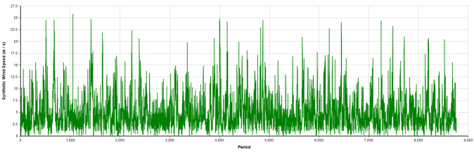
Looking at the second period, the wind is in state 6 (scroll up to the state simulation table).  From the Enter States variable, state 6 has a low state speed of 5 and an high state speed of 6.  Along with a random variable of 0.236 we see that the simulated wind speed is 5.236 (= 5 + 0.236 *(6 – 5) ).  Here is a chart of run 37’s generated wind speeds over 8,759 hours:

Comparisons

I won’t get into any formal statistical checks of the model, see Shamshad et al (2005) for various hypothesis tests.  But let’s compare the histogram of the data and a randomly chosen simulation run:

This looks like a good fit, which is what we expect since the Markov chain will reproduce the underlying probability mass function. However as mentioned above we do need more than a year of data to capture the higher wind speeds due to the infrequency with which they occur.  The statistics for this run and the historical data are below:

Again, as expected they are quite close.  Note that different runs of the model will have slightly different statistics, particularly with respect to the extreme values. But this is also to be expected since the time series of generated wind speeds will be different for each run of the model.

The last chart to look at is the limit distribution.  This represents the long term frequency of the wind speed being in each state:

So overall the Markov chain does provide a nice and simple way to simulate wind speed time series.

Limitations of Markov Models

The focus of the model presented in this post is to generate wind speed information for evaluating the financial feasibility of a wind energy project. However, as Brokish and Kirtley (2009) convincingly argue, when studying a wind resource to size energy storage or spinning reserves Markov chains may not be an effective simulation method. The reason is that the Markov chain may not capture the autocorrelation between subsequent wind speeds at smaller time increments.  They argue that Markov chains are effective for time increments above 15 to 40 minutes depending on the order of the chain.  Since we are focused on hourly wind speed data this model should not be impacted.

Conclusion

Generating accurate synthetic time series of wind speeds is an important task in creating a financial model for a wind energy project.  Following the literature I used a simple first order Markov chain to do just that.  However there are a number of ways to extend the model that may generate more accurate wind speeds for a given wind resource.  The first is to add seasonality as Karatepe and Corscadden (2013) suggest, since wind speeds depend on the season.  Another approach is to use a higher order Markov chain, which incorporates not just the present hour but also previous hours when estimating state transition probabilities. Higher order chains have the advantage of being more accurate at lower time scales, but also greatly increase the computational cost.  However for a preliminary investigation of a wind resource a first order Markov chain, as used in this post, should suffice for many locations.

Once the hourly wind speed series has been generated, a financial modeler can then aggregate from hourly power production to monthly and finally yearly power production.  With this power production information an accurate cash flow model can be created.  But I leave that for another post.

References

1. Aksoy, H., Z. F. Toprak, A. Aytek, N. E. Ünal (2004): “Stochastic generation of hourly mean wind speed data,” Renewable Energy, 29(14), 2111-2131.
2. Brokish, K., J. Kirtley (2009): “Pitfalls of modeling wind power using Markov chains,” 2009 IEEE/PES Power Systems Conference and Exposition, 1-6
3. Jain, P., (2016): Wind Energy Engineering, Second Edition, McGraw-Hill Education.
4. Karatepe, S., K. W. Corscadden (2013): “Wind Speed Estimation: Incorporating Seasonal Data Using Markov Chain Models,” ISRN Renewable Energy, vol. 2013, Article ID 657437, 9 pages.
5. Sahin, A. D., Z. Sen, (2001): “First-order Markov chain approach to wind speed modelling,” Journal of Wind Engineering and Industrial Aerodynamics, 89(3), 263-269.
6. Shamshad, A., M. A. Bawadi, W. M. A. Wan Hussin, T. A. Majid, S. A. M. Sanusi (2005): “First and second order Markov chain models for synthetic generation of wind speed time series,” Energy, 30(5), 693-708.